Open access

Research Article

18 March 2026

Comparison of two-stage methods for count data in Mendelian randomization: a simulation study

Authors: Mary Appah https://orcid.org/0000-0001-6406-6269 [email protected], Riku Takei, Vinodh Srinivasasainagendra, Sandeep C Vejandla, Richard J Reynolds, Tony R Merriman, and Hemant K TiwariAuthor Info & Affiliations

Publication: Journal of Comparative Effectiveness Research

Volume 15, Number 4

https://doi.org/10.57264/cer-2025-0081

PDF

Abstract

Aim: Mendelian randomization (MR) is an instrumental variable (IV) method that utilizes genetic variants to establish causality between risk factors and outcomes in observational studies. These methods were primarily developed under assumptions appropriate for continuous or approximately normally distributed variables. However, in many biomedical and clinical studies, exposures and outcomes are naturally recorded as counts, such as the number of disease episodes or clinical events. Despite this, two-stage MR methods are applied to count data without a clear understanding of their validity under such settings. While individual-level MR methods like two-stage predictor substitution (TSPS) and two-stage residual inclusion (TSRI) are common, their comparative performance for count exposures and outcomes remains unclear. Materials & methods: We conducted the first systematic evaluation of TSPS and TSRI for count data using Poisson and negative binomial models across realistic MR scenarios. Simulations varied instrument strength (IS), confounding, sample size and also focused on invalid instruments. Performance was assessed by bias, root mean square error (RMSE), 95% confidence interval (CI) coverage, CI width and Type I error rate. To demonstrate practical application, we applied these methods to investigate the causal relationship between alcohol consumption and gout attacks using empirical data. Results: Our results revealed that across all scenarios, TSRI with the Poisson model produced the most stable estimates with lower bias and RMSE. TSRI achieved near-nominal coverage and narrower CI across varying IS and confounding levels, maintaining Type I error close to 0.05. IS significantly impacted performance, with IS = 0.5 yielding estimates closer to the true values, while weaker instruments (IS = 0.1) led to higher RMSE and bias. Increasing sample size in the presence of invalid and weak genetic variants increased the bias. In additional simulations with multiple weak instruments, TSRI continued to outperform TSPS, yielding lower bias or RMSE, narrow CI width and near-nominal coverage across sample sizes. In our application, alcohol consumption was causally associated with an estimated 11.6–12.7% increase in the expected number of gout attacks per year per unit increase in alcohol intake, although the presence of an invalid single nucleotide polymorphism likely biased this estimate. Conclusion: This study advances MR methodology by clarifying how TSPS and TSRI behave with count exposures and outcomes, providing practical guidance for valid instrument selection and reliable causal inference in MR studies involving count data.

Plain language summary

What is this article about?

This study compares two methods used to study whether an exposure causes an outcome, especially when the outcome is a count (like the number of gout attacks). These methods use genetics to help understand cause-and-effect relationships in health research. The goal was to see which method works better when dealing with this kind of data.

What were the results?

Using simulations, we found that the two stage residual inclusion method with a Poisson model gave more accurate results, especially when strong genetic variants were used. When the genetic variants were weak or not valid, the results became more biased. In a real-world example, we looked at whether alcohol consumption causes gout attacks. We found a link but also showed that using an invalid genetic variant could lead to misleading conclusions.

What do the results mean?

This study shows that choosing strong and valid genetic variants is very crucial when using these methods to study cause and effects. Using weak or invalid ones can produce biased results, even if a large amount of data is available. This is important for researchers using genetic data to make health-related decisions.

The gold standard for testing a scientific hypothesis to infer causality in clinical research is usually done with randomized control trials (RCT) [1–5]. These trials involve assigning treatments and placebo to subjects at random and then comparing the average outcome of subjects between groups [6]. The goal of these trials is to determine whether the treatment has a causal effect on the outcome of interest, which could be a disease state, biomarker, symptom improvement or other health-related endpoint. However, RCTs cannot always be performed because they can be costly, impractical, or even unethical [3,4,7,8]. In circumstances where RCTs cannot be conducted, instrumental variable (IV) methods can be used to evaluate causality [5]. These methods are alternate causal analysis methods used in observational studies to address the issue of confounding and reverse causation if certain assumptions are satisfied [9]. IV methods were first introduced in econometrics as a way to address endogeneity issues in observational research [10]. Endogeneity is a situation in which an independent variable is correlated with the error term in a regression analysis [10]. This scenario breaches a fundamental assumption of regression analysis, exogeneity, which is crucial for ensuring that changes in the dependent variable are properly linked to the independent variables rather than to unobserved or omitted confounding factors [11]. For this reason, fitting a regression model will result in an estimated coefficient being biased and inconsistent, and the model will not provide reliable causal estimates.

The general assumptions of IV methods are that the IV must be associated with the exposure of interest (relevance), the IV should only be related to the outcome of interest through the exposure under study (exclusion restriction), and the IV should not be associated with confounders of the exposure–outcome relationship (independence) [12–15]. These assumptions are summarized in Figure 1. The most difficult aspect of IV analysis is identifying an appropriate IV [5,12,16]. However, if an IV is found that satisfies these assumptions, causality can be established. There are several sources of IVs, each with distinct characteristics and applications, but in the context of this paper, we focused on using genetic variants as IV, termed Mendelian randomization (MR). Genetic variants are randomly transmitted during reproduction and are generally unaffected by environmental influences [17]. MR uses the fact that genotypes are not generally susceptible to reverse causation and confounding because of their fixed nature and Mendel’s second law of inheritance [18–20]. Therefore, they are less likely to be subject to confounding, making them valuable tools for causal inference. This situation draws a parallel to an RCT, where the randomly inherited genetic variant plays a role akin to random treatment assignment, and the risk allele functions as the treatment received. The genetic variants divide the population into subgroups so that any differences seen in the outcome between these groups can be attributed to a causal effect of the risk factor of interest, provided the assumptions of IV are satisfied [21].

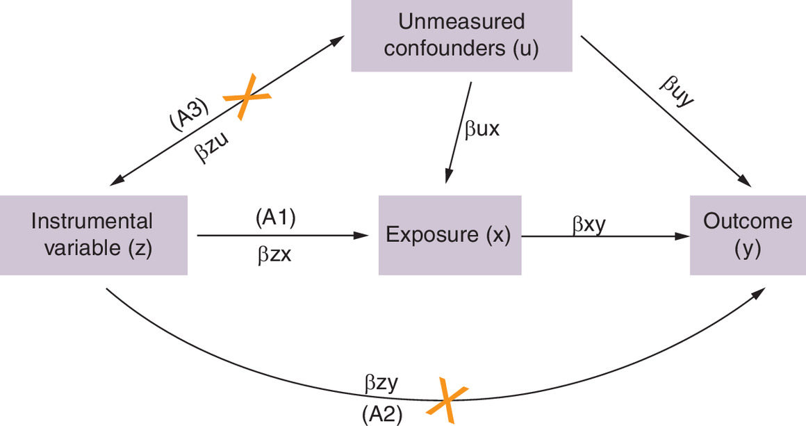
Visualization of a complex neural network architecture used in the research study. — Figure 1. Directed acyclic graph showing the core instrument variable assumptions in Mendelian randomization.
Directed acyclic graph (DAG) illustrating the core assumptions (A1–A3) of Mendelian randomization. The red cross on the arrow from Z to Y indicates that the IV (instrument variable) should influence Y only through X, ensuring the exclusion restriction assumption (A2) holds. The red cross on the arrow from Z to U signifies that the IV should not be associated with U of the X–Y relationship, ensuring the independence assumption (A3) holds.
A: Assumption.

Genetic variants are differences in DNA that contribute to the genetic diversity among individuals [22]. The most common type of genetic variant is a single nucleotide polymorphism (SNP), which is often used as an IV in MR. The purpose of using genetic variants as IVs in MR studies is to address the issue of unmeasured confounding and it is therefore imperative that a valid and appropriate genetic variant is selected in MR studies. Choosing a genetic variant that is not strongly associated with the exposure causes a bias that is referred to as weak instrument bias [23,24]. The association between the genetic variant and exposure is evaluated using linear regression to determine its strength [20,25]. For this reason, choosing a weak instrument as an IV will explain a relatively small proportion of the variance in the exposure. The most common metric used is F-statistic, where a value greater than 10 is considered a strong relationship between the genetic variant and exposure [23,26–28]. However, it is unknown if this metric still holds for non-linear relationships.

There are several methods developed for MR estimation, but two MR estimation methods are of interest: the two-stage predictor substitution (TSPS) and the two-stage residual inclusion (TSRI). These methods were selected because of their widespread use and ease of implementation in any software that can be used for regression analysis. Originally, these methods were developed for continuous variables, but more recently, TSPS has been extended to accommodate other types of data. While TSPS produces accurate and consistent causal effect estimates, it often underestimates uncertainty through its standard errors because it fails to fully account for first-stage variability in the second-stage model [10,29]. To address this limitation, the TSRI method was adapted from econometrics to be used in the context of MR. Unlike TSPS, TSRI incorporates first-stage variability into the second-stage model, resulting in more accurate standard errors [10]. For linear models, both methods yield identical causal effect estimates [30], but simulation studies have shown that TSRI performs better in nonlinear settings when outcomes are binary [10,31]. However, questions remain about which of the two methods is more appropriate for count variables.

In many MR studies, exposures and/or outcomes of interest are measured as count variables, such as the number of disease episodes or clinical events over time. Nevertheless, TSPS and TSRI are often applied to such data types despite limited evidence on how these methods perform when the key assumptions, such as linearity and normality, are violated. This lack of evaluation creates uncertainty about the reliability of causal estimates obtained from two-stage MR methods when used with count data.

Count variables take on discrete values like 0, 1, 2, 3, etc., representing the number of times an event occurs during a fixed period. It can take only nonnegative numbers. The distribution of these variables is mostly positively skewed with a peak at zero, hence not normally distributed, and therefore Poisson models have been used to model such data [32]. Poisson regression assumes that the mean and variance are equal; however, this assumption is often unrealistic in practice, leading to overdispersion when the variance exceeds the mean. To address this issue of overdispersion, negative binomial distributions have been suggested as a more appropriate model [32,33].

This study aims to address this gap by comparing the performance of TSPS and TSRI for count data using Poisson and negative binomial regression. We concentrated more on conditions where instrument strength (IS) is weak and the instrument is not appropriate, since it might not always be practical to find a strong and appropriate IV. We compared these methods by simulating data with a variety of parameters in different scenarios (Table 1) and assessed bias, RMSE, CI coverage, CI width and Type I error rate for null causal effect as performance metrics. We also illustrate the application of these methods by determining whether total alcohol consumption causes gout, emphasizing the dangers of making causal conclusions when using invalid IVs.

Table 1. Description of simulation scenarios used in evaluations of two-stage methods for varying instrument strength.

Scenario	Description	Parameter settings
1	Null causal effect Moderate sample size Varying instrument strength	β_xy = 0 n = 1000 β_zx varying from 0.001 to 1.0 β_x0 = 0, β_y0 = 0, β_u0 = 0, β_zu = 0, β_zy = 0, β_ux = 0.5, β_uy = 0.5 n_sims = 1000
2	Positive causal effect Moderate sample size Varying instrument strength	β_xy = 0.4 n = 1000 β_zx varying from 0.001 to 1.0 β_x0 = 0, β_y0 = 0, β_u0 = 0, β_zu = 0, β_zy = 0, β_ux = 0.5, β_uy = 0.5 n_sims = 1000

Although TSPS and TSRI have been studied in econometric contexts, their comparative performance has not been systematically evaluated within MR, particularly when both exposure and outcome are count variables. This study extends previous econometric findings to MR settings by incorporating weak and invalid instruments, varying confounding and sample size. It further demonstrates the practical implications through a reanalysis of the alcohol–gout relationship.

Materials & methods

To evaluate the performance of TSPS and TSRI for count data, we considered a setting with individual-level data consisting of an exposure (X), an outcome (Y) and a single nucleotide polymorphism (SNP) as our IV. In our framework, both X and Y were treated as count variables, while Z was assigned as an IV that takes on values 0, 1 or 2. The two-stage approaches were implemented under this setup, and their performance was assessed using the following performance metrics: bias, root mean square error (RMSE), coverage, 95% CI width and Type I error.

Two-stage predictor substitution (TSPS)

This method is called ‘two-stage’ because its estimation is conducted in two sequential steps. In the first stage, genetic variant is used as instrument to predict the exposure of interest. The predicted exposure values are then used in the second stage to estimate the causal effect of the exposure on the outcome using Poisson or negative binomial models. However, TSPS often underestimates standard errors because it does not fully account for the variability that occurs in the first stage model.

Two-stage residual inclusion (TSRI)

TSRI better handles the underestimation of the standard errors by making sure that the variability in the first stage is carried over and accounted for in the second stage [10]. Therefore, the standard errors become more accurate, giving a better picture of the uncertainty in the estimates. Like TSPS, TSRI involves two-stage systems of Poisson or negative binomial models. The first stage is the same as that of TSPS. From the first stage model, the residuals are extracted and used as a covariate in a second-stage Poisson regression model.

Simulation

To compare the performance of TSPS and TSRI with count data and different regression models, we conducted a simulation study with different scenarios and parameter values to mimic a realistic setting. The description of the simulation scenarios is presented in Table 1. For each individual i, we simulated data on a genetic variant Z_i, a modifiable exposure X_i, an outcome variable Y_i and an unmeasured confounder U_i. We estimated the causal effect of the exposure on the outcome using one SNP. The SNP variable Z_i was simulated to represent the number of minor alleles present in a diploid genotype, following a binomial distribution Binomial (2, 0.2). This distribution naturally produces three possible values (0, 1, or 2) corresponding to the possible counts of minor alleles across the two chromosomal copies, with 0.2 representing the minor allele frequency in the population.

A confounder U was generated as a normally distributed variable, with the mean determined by an intercept, an effect from the SNP, and an error term, such that

U = β_{U 0} + β_{Z U} Z + ε_{U}

The exposure variable X was modeled as a Poisson random variable with a mean parameter determined by an exponential function incorporating the SNP effect, the confounder, and an error term:

β_{X 0} + β_{Z X} Z + β_{U X} U + ε_{X}

X \sim P o i s s o n (e x p (β_{X 0} + β_{Z X} Z + β_{U X} U + ε_{X}))

The outcome variable Y was also modeled as a Poisson random variable with a mean dependent on the exposure, SNP, confounder, and error term:

{Y \sim P o i s s o n (e x p (β}_{Y 0} + β_{Z Y} Z + β_{X Y} X + β_{U Y} U + ε_{Y}))

where ε_U ε_X ε_Y ∼N (0,1)

The introduction of the variable β_ZY represents a violation of Assumption 2 (exclusion restriction) in Figure 1. In most simulation scenarios (scenarios 1–4), β_ZY is set to 0, as expected in a valid MR. Only in scenario 5 (Table 3), β_ZY is set to 0.2, indicating a violation of the exclusion restriction assumption. Additionally, β_ZU corresponds to a violation of Assumption 3 (independence) and this parameter is set to zero in all scenarios. The simulation equations were written in a general form to accommodate the specific settings used in each scenario.

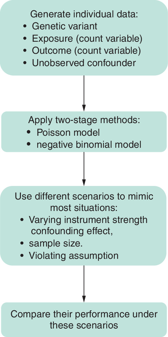
For each scenario, we varied parameters to assess the robustness of the method under different conditions as shown in Tables 1–3. Simulations were repeated using 1000 datasets (n_sims) across a range of parameter values to ensure a thorough assessment of the method's accuracy and precision in different real-world settings. For scenarios with non-null causal effect, 1000 iterations were used to construct 95% CIs via percentile bootstrapping with 500 resamples. For evaluating the Type I error rate under the null hypothesis, simulations were performed using 10,000 iterations to provide stable estimates. All simulations and statistical analyses were conducted in R using the base R glm function for Poisson regressions and the MASS package for negative binomial regressions (glm.nb). Figure 2 provides a conceptual overview of the simulation process and performance evaluation framework.

Table 2. Description of simulation scenarios used in evaluations of two-stage methods for varying confounding effects.

Scenario	Description	Parameter settings
3	Null causal effect Moderate sample size Varying confounding effect	β_xy = 0 n = 1000 β_zx = 0.1 β_x0 = 0, β_y0 = 0, β_u0 = 0, β_zu = 0, β_zy = 0, β_ux, β_uy varying from 0.05 to 1.2 n_sims = 1000
4	Positive causal effect Moderate sample size Varying confounding effect	β_xy = 0.4 n = 1000 β_zx = 0.1 β_x0 = 0, β_y0 = 0, β_u0 = 0, β_zu = 0, β_zy = 0, β_ux, β_uy varying from 0.05 to 1.2 n_sims = 1000

Table 3. Description of simulation scenarios used in evaluations of two-stage methods for sample size and violation of assumption (A2).

Scenario	Description	Parameter Settings
5	Positive causal effect weak instrument strength Varying sample size Violation of Assumption 2 in Figure 1	β_xy = 0.4 β_zx = 0.1 n varying from 100 to 5000 β_x0 = 0, β_y0 = 0, β_u0 = 0, β_zu = 0, β_uy = 0.2, β_uz = 0.5, β_uy = 0.5 n_sims = 1000

Figure 2. Conceptual overview of the simulation process and performance evaluation framework.

Multiple SNP setting

In addition to the single SNP scenario, we evaluated a setting with multiple weak genetic instruments to better reflect common MR practice. We generated 4 SNPs, each with a minor allele frequency of 0.2, Z_j ∼ Binomial (2, 0.2) for j = 1, …, 4, and formed an unweighted allele score

Z = \sum_{j = 1}^{4} Z_{j}

.All other components of the data generating process were identical to the single SNP setting. We varied the sample size (n = 100, 500, 1000, 2500, 5000), used an IS of 0.1, a confounding effect of 0.5 and a true causal effect of 0.4.

Results

We evaluated the performance of TSPS and TSRI with Poisson and negative binomial regression to identify the most suitable option for specific conditions. Specifically, we varied IS, confounding effect, and sample size with violation of assumption 2 as shown in Tables 1–3, respectively. Figure 3 demonstrates the effect of the exposure on the outcome for scenarios 1 (Figure 3: Top row) and 2 (Figure 3: Bottom row) with varying IS across five levels (0.001, 0.01, 0.1, 0.5 and 1). The corresponding F-statistics are 1.21, 1.02, 2.79, 73.10 and 247.52. For the null causal effect, the relationship between IS and the bias follows an inverse relationship across all the two-stage methods regardless of the distribution used. With IS values of 0.5 and 1, both null and positive causal effect estimates were closer to the true values across all two-stage methods, regardless of whether Poisson or negative binomial regression was used.

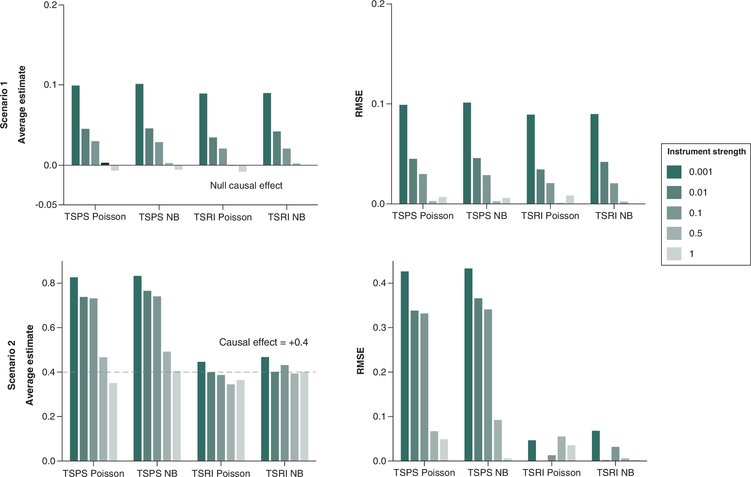
Effect of instrument strength on causal estimate accuracy for null and positive effects, showing inverse relationship across methods. — Figure 3. Average causal effect and root mean square error for a null (scenario 1) and positive causal effect of 0.4 (scenario 2) varying instrument strength.
The dotted line indicates the true causal effect.
NB: Negative binomial; RSME: Root mean square error; TSPS: Two-stage predictor substitution; TSRI: Two-stage residual inclusion.

To assess the strength using the F-statistics, IS of 0.5 and 1 had an F-statistic greater than 10 which is considered a strong instrument while the others (0.001, 0.01 and 0.1) had an F statistic less than 10 indicating a weak instrument. With a positive causal effect of 0.4, TSRI negative binomial models demonstrated the most stable performances, maintaining relatively consistent estimates across different IS values. TSPS Poisson and TSPS negative binomial models exhibited greater deviation from the null. This suggests that weaker instruments introduce bias and higher RMSE, reinforcing the importance of selecting strong instruments for accurate causal estimates using two-stage methods.

Similarly, the inverse relationship between IS and the average estimate remained consistent for the positive causal effect (scenario 2). However, certain patterns were more prominent: TSRI methods demonstrated superior performance, especially when applied to a negative binomial distribution, where they produced more stable estimates. Weaker IS continued to yield higher RMSE, reinforcing the need for strong instruments to minimize bias and improve reliability.

Additional performance metrics (Supplementary Tables 2 & 3) showed that coverage remained near the nominal 95% level for strong instruments but dropped slightly for weak ones. Type I error was well controlled (∼0.05) under strong instruments and very small (<0.01) under weak instruments. Confidence-interval width decreased as IS increased, and TSRI generally achieved narrower intervals than TSPS.

In Figure 4 where we varied the confounding effects, the influence of confounding effects on causal estimates was pronounced: as confounding strength increased, the difference between the estimated average causal effect and true causal effect also increased. The corresponding F-statistics are 3.54, 3.11, 2.79, 2.93 and 2.33 corresponding to increasing confounding effects (0.05 to 1.2). TSRI methods outperformed TSPS methods, particularly under a Poisson model, where the estimates remained more stable. When confounding is minimal for null true causal effect (scenario 3), all methods produce estimates close to zero, suggesting minimal bias. However, as the confounding effect increases, the bias becomes more evident, which shows upward deviations from the null. The RMSE increases with higher confounding effects, particularly for all methods except TSRI Poisson which exhibits minimal deviation from the true null causal effect and lowest RMSE values. In scenario 4, the TSPS Poisson and TSPS NB methods consistently overestimate the causal effect, particularly under stronger confounding effects. In contrast, TSRI Poisson provides estimates closer to the true value. TSRI Poisson consistently underestimates the effect but performs better than TSPS approaches. The RMSE remains highest for TSPS Poisson and TSPS NB, with increasing instability as the confounding effect increases. Overall, the TSRI Poisson method exhibited the most stable estimates despite increasing confounding effects. TSPS methods and the TSRI negative binomial method were more sensitive to confounding, with greater deviations from the true causal effect at a confounding effect of 1.2.

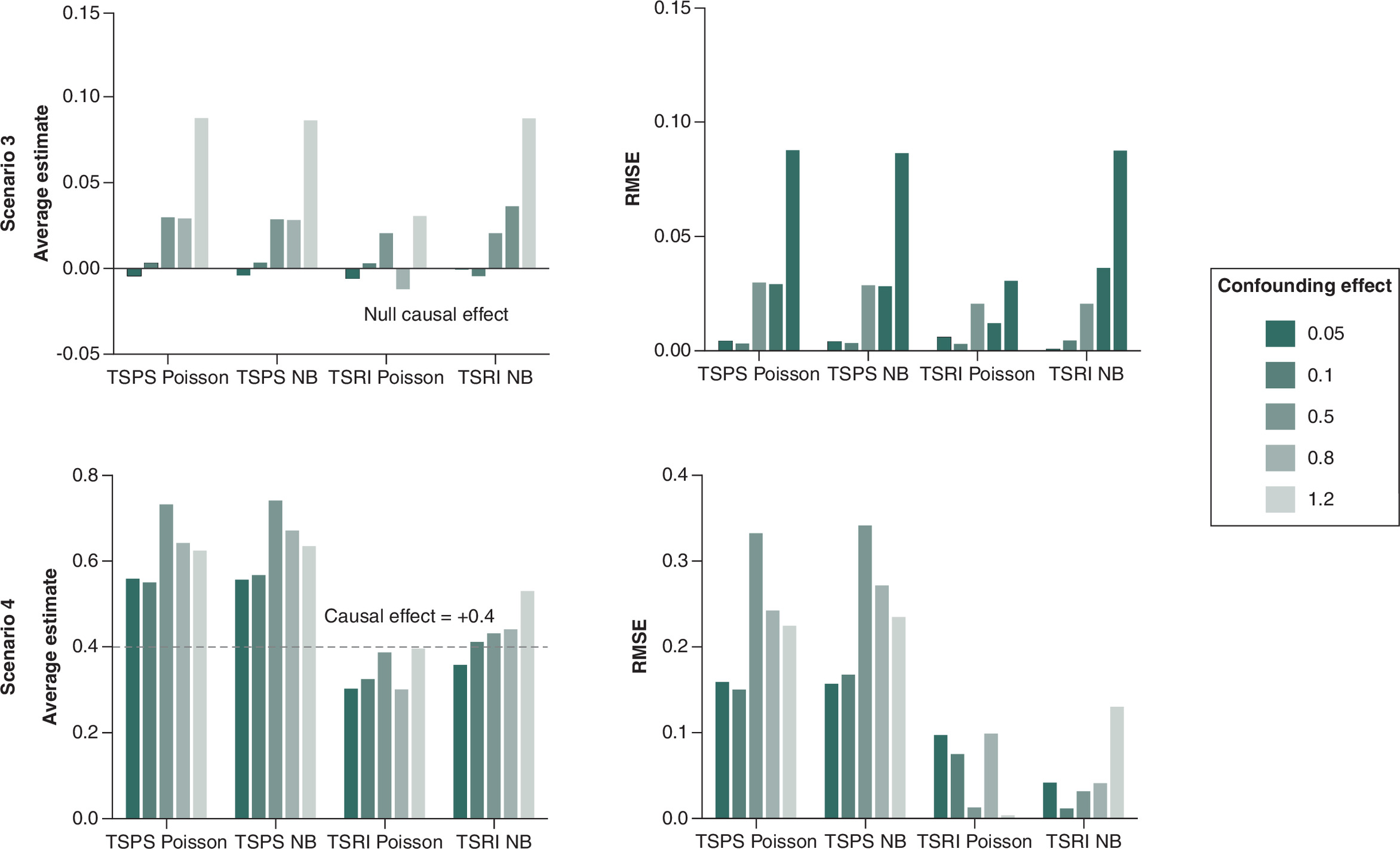
Comparison of average causal effect estimates under varying confounding effects, showcasing superior performance of TSRI methods in stability and accuracy. — Figure 4. Average causal effect and root mean square error for a null (scenario 3) and positive causal effect of 0.4 (scenario 4) with varying confounding effects.
The dotted line indicates the true causal effect.
NB: Negative binomial; RSME: Root mean square error; TSPS: Two-stage predictor substitution; TSRI: Two-stage residual inclusion.

Expanded metrics (Supplementary Tables 4 & 5) confirmed these trends: coverage stayed near 95% when confounding was weak but declined slightly with stronger confounding. Type I error remained well controlled (∼0.006–0.011), and TSRI Poisson exhibited narrower confidence intervals and more stable coverage than other methods.

In Figure 5, we evaluated the effect of sample size (100–5000) in estimating the causal effect (+0.4) and MR assumption violations. The F-statistics for these sample sizes are 1.11, 1.68, 2.79, 7.04 and 14.66, demonstrating a transition from extremely weak instruments at small sample sizes to moderate strength at larger sample sizes. With smaller sample sizes (100 and 500), all methods exhibit overestimation, with TSPS Poisson and TSPS NB performing the worst. As the sample size increased, the bias also increased. Since increasing the sample size did not reduce bias, selecting appropriate genetic variants in MR studies is crucial for minimizing bias.

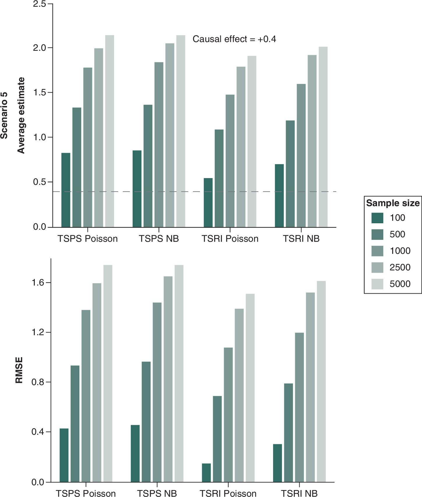
Effect of sample size on estimating causal effects and MR assumption violations, showing transition from weak to moderate to strong instrument strength. — Figure 5. Average causal effect and root mean square error for a positive causal effect of 0.4, varying sample size and violation of exclusive restriction assumption.
The dotted line indicates the true causal effect.
NB: Negative binomial; RSME: Root mean square error; TSPS: Two-stage predictor substitution; TSRI: Two-stage residual inclusion.

Supplementary Table 6 adds context for this scenario: coverage declined markedly as sample size increased, falling below 0.80 for TSPS and only slightly higher for TSRI. Type I error inflated at larger n, and CI width narrowed without improved accuracy. This pattern reflects bias from the invalid instrument rather than reduced efficiency larger samples produced more precise but still biased estimates. These results emphasize that increasing sample size cannot offset bias from invalid or weak instruments.

Results from the multiple weak-instrument scenario are summarized in Supplementary Table 1. The F-statistic for the smallest sample size (n = 100) was 3.35, indicating weak instruments, whereas for larger samples (n = 500) the F-statistics exceeded 10, reflecting stronger instruments. Bias and RMSE decreased with increasing sample size, and coverage remained close to nominal 95% across all n. TSRI consistently produced smaller bias, lower RMSE and narrower CIs than TSPS under both Poisson and negative binomial models. The similarity between Poisson and NB results suggests that overdispersion had little influence in this setting.

Application: Causal association between alcohol consumption and gout using MR.

Gout is a common form of inflammatory arthritis caused by the deposition of monosodium urate crystals in joints of the body accompanied by an extremely painful immune response [34,35]. It is the most prevalent inflammatory arthritis [35]. Epidemiological studies have consistently associated alcohol consumption with an increased risk of gout [36,37], likely due to the role of alcohol in raising serum uric acid levels through purine metabolism and renal excretion pathway [38,39]. While these studies suggest a link, we cannot determine whether the relationship is causal, as observational designs are prone to confounding and reverse causation.

Recent findings by Chuah et al. have further highlighted the complexity of this relationship, showing that the effect of genetic variants on serum urate and gout risk may depend on alcohol consumption [40]. In their study of European ancestry participants, variants at the ADH1B and MLXIPL loci were significantly associated with gout risk only among alcohol consumers, underscoring a gene–environment interaction that complicates causal inference. These findings support the need for methods like MR, which uses genetic variants as instrumental variables to infer causality.

In this study, we applied MR to assess the causal role of alcohol in gout while illustrating the impact of instrument selection on MR results. Specifically, we explore the consequences of using a potentially invalid SNP as an instrument in MR studies. We compared TSPS and TSRI using both Poisson and negative binomial models using data from a European cohort in a published study that investigated the interaction between alcohol consumption and urate-associated genetic variants in gout risk [41]. This data was accessed on 1 January 2025 for secondary analysis. Written informed consent was obtained for all participants as per the original study protocol. The data was fully anonymized before being accessed for secondary analysis in this study, and no additional consent was required. The study genotyped 29 SNPs across various loci associated with serum urate levels and gout, analyzing their interaction with alcohol exposure. From this dataset, we specifically selected rs780094 in the GCKR gene as an instrument for alcohol consumption. This SNP was identified as highly significant in the study (Table 2 from [41]) and was found to interact with alcohol consumption in European participants (p = 1.5 × 10^-4). However, the study also reported that alcohol exposure eliminated the genetic effect of rs780094 on gout risk, suggesting that this SNP may violate the exclusion restriction assumption which is a fundamental requirement for a valid MR instrument. In addition, rs780094 has been associated with multiple other phenotypes, such as triglyceride levels, glucose metabolism and metabolic traits, which are themselves known risk factors for gout [42,43]. This pleiotropic effect implies that rs780094 may influence gout through biological pathways other than alcohol consumption, leading to biased causal estimates when used as an instrument.

We estimated the causal effect of total alcohol consumption (exposure) on the number of gout attacks (outcome). Both exposure and outcome are count variables and by applying rs780094 in our real-data MR analysis, we can evaluate if using a genetically invalid instrument can lead to bias. The genetic variant (rs780094) was treated as a categorical variable coded as 0, 1 or 2, representing the number of risk alleles. Total alcohol consumption was measured as the self-reported number of alcoholic drinks consumed per week. Participants reported their average weekly intake across different types of beverages, with standard drink definitions applied: one beer = 330 ml, one glass of wine = 200 ml, one serving of spirits = 30 ml and one other alcoholic drink = 330 ml. The total weekly alcohol intake was calculated as the sum of these values, with a mean (SD) of 7.68 (11.39) standard drinks per week. Gout attacks were assessed by asking participants to report the number of acute gout flares experienced over the past 12 months. This was used as the outcome variable, expressed as the number of gout attacks per year, with a mean (SD) of 4.92 (9.57) attacks per year. We excluded participants who had missing data for either exposure or outcome or both. The final analysis included 949 participants, of whom 84.3% were men.

Table 4 presents the effect estimate, standard error, and p values of the two-stage methods with the Poisson and negative binomial model. In addition, we analyzed the data using the regression of the outcome Y on the exposure X, which is referred to here as Naive. This method is affected by confounding and therefore, causal inferences cannot be made. Some possible confounders of the relationship between alcohol and gout include but are not limited to, kidney function, obesity and dietary factors such as consumption of red meat. The results showed that the naive method yielded nonsignificant null effects for both Poisson and negative binomial models (p = 0.8). This suggests that alcohol may not be associated with gout. On the other hand, both two-stage methods indicate a significant positive causal effect, all p < 0.05. Our MR analysis suggests that genetically predicted alcohol consumption is associated with an approximately 11.6–12.7% increase in the expected number of gout attacks per year per unit increase in alcohol intake. However, due to the use of an invalid SNP, this result is likely biased as was observed in the simulation results, highlighting the risks of using weak or invalid instruments in MR.

Table 4. Estimate, standard error and p-value from data application.

Method	Estimate	Standard error	p-value
Naive: Poisson	0.0003	0.0013	0.8000
Naive: negative binomial	0.0002	0.0042	0.9580
TSPS: Poisson	0.1122	0.0139	<0.001
TSPS: negative binomial	0.1206	0.0503	0.0165
TSRI: Poisson	0.1125	0.0140	<0.001
TSRI: negative binomial	0.1217	0.0504	0.0158

TSPS: Two-stage predictor substitution; TSRI: Two-stage residual inclusion.

Discussion

MR uses genetic variants as an IV to infer causal relationships between exposure and outcome. However, when the appropriate SNP(s) are not chosen for MR studies, it results in misleading and inaccurate conclusions about causality. In this study, we compared the two-stage methods, that is TSPS and TSRI using the Poisson and negative binomial model.

Our simulations assessed different levels of IS, confounding effect and sample size with weak and invalid IV and their effect on causal estimates. In Figure 3, an IS of 0.001 with F-statistics of 1.21, far below the conventional threshold of 10, led to a causal estimate that deviated significantly from the true effect. We observed that an IS value of 0.5 provided a more accurate causal estimate than IS = 1, despite having a lower F-statistic (73.104 vs 247.52). This aligns with the findings by Burgess and colleagues [23], who found that excessively large F-statistics lead to biased causal estimates, pulling them toward the observational association and reducing their standard errors. In the same study, the authors questioned the widely accepted rule of thumb that an F-statistic greater than 10 ensures strong IV-exposure associations, since this may be misleading if the F-statistic is too large. For the positive causal effect scenario, we observed a similar trend in bias. When IS was weak, the causal estimate approached the observational estimate of the exposure–outcome association, which is biased due to confounding [44]. The F-statistic, commonly used to measure IS depends on sample size (n), the number of instruments (k) and the proportion of variance explained by the IV (R²), as defined by

F = (\frac{n - k - 1}{k}) (\frac{R^{2}}{1 - R^{2}})

[45]. It is widely accepted that increasing sample size can artificially inflate F-statistics even when R² is small [46]. In our study, we varied sample size in scenario 5 when assumption 2 (the exclusion restriction assumption) was violated (Figure 5) and as sample size increased, the average causal estimate deviated from the true causal effect. While increasing sample size raised the F-statistic, it also increased the bias due to weak instrument effects and violations of assumption 2. This clearly shows that relying solely on F-statistics to assess IV-exposure strength is insufficient, particularly in nonlinear models [47]. This has been reported in empirical studies where observed F-statistics > 10 do not necessarily reflect the true strength of an instrument due to sampling variation [23] and weak instrument bias.

A more robust approach that incorporates additional metrics and sensitivity analyses is needed to properly evaluate IS, particularly in nonlinear MR studies. Including several genetic variants can improve the accuracy of estimates by capturing more variation in the exposure. However, if some of these variants are invalid or influence the outcome through pathways other than the exposure, they can introduce bias instead of reducing it [20,27,48,49], making instrument selection crucial in MR studies.

Our real-data application investigated the causal effect of alcohol consumption on the number of gout attacks. We estimated the causal effect using TSPS and TSRI with both Poisson and negative binomial models, which produced similar positive estimates. However, these estimates were unreliable because the SNP used violated key MR assumptions. Comparing this scenario to our simulation results (Figure 5), we observed substantial bias across all methods and sample sizes, with bias as the sample size increased. A recent MR study [50] investigated whether alcohol consumption causally increases the risk of gout but found no significant causal effect. Hence conclusions can be misleading when the appropriate SNP is not used. Additionally, previous studies [51,52] have shown that TSPS estimators tend to be biased toward the Ordinary Least Squares (OLS) estimate, with standard errors smaller than the bias. When instruments are weakly correlated with the exposure, conventional asymptotic results fail even in large samples [23] as observed in our simulations (Figure 5).

Earlier studies [10,53] proposed using the TSRI method for nonlinear models, and our simulations confirm its superiority over TSPS. Similarly, other simulation studies [10,54–56] have also demonstrated that TSRI is generally consistent for nonlinear models, whereas the TSPS method is not.

Our findings support this conclusion, showing that TSRI is less biased than TSPS when working with count data. This study highlights key challenges in MR, including weak instrument bias, the limitations of F-statistics, and the importance of instrument selection. Our findings emphasize the need for alternative methods beyond F-statistics to assess IV strength, particularly in nonlinear settings. The results also confirm that TSRI performs better than TSPS for count data, reinforcing its value in MR studies involving Poisson and negative binomial models. Future research should explore alternative approaches to IS assessment in nonlinear MR models.

While this study provides insights into the performance of two-stage methods under varying instrumental strength, confounding effects and assumption violations, several limitations should be noted. First, this study demonstrates the impact of IS on bias and RMSE using a single SNP but does not explore using multiple SNPs where each explains a small proportion of the exposure variance.

In this study, we used the Poisson model as the true data-generating process for the count variables and applied both Poisson and negative binomial models for estimation to account for potential overdispersion. However, we did not explore other distributional features commonly seen in real-world count data, such as zero inflation or the use of alternative distributions like the gamma distribution. In addition, we did not investigate the effects of very small or extremely large sample sizes, nor did we examine violations of other instrumental variable assumptions beyond the one related to instrument validity. Our primary focus was on evaluating how using an invalid genetic variant, specifically violating one of the core MR assumptions impacts causal effect estimates. As such, the generalizability of our findings may be limited, as different data characteristics or assumption violations could lead to different results.

Conclusion

This study highlights several key insights into the performance of two-stage methods for causal inference. IS plays a crucial role, as weaker instruments lead to increased bias, wider CI width and higher RMSE, emphasizing the importance of strong and valid instruments for accurate estimation. Among the methods evaluated, TSRI models particularly those based on the Poisson distribution demonstrated greater stability and resilience to confounding compared with negative binomial-based models. Additionally, confounding effects exacerbate bias, with TSPS methods showing greater sensitivity and higher RMSE, whereas TSRI methods maintain greater robustness. Sample size also significantly impacts estimation, with MR assumption violations leading to highly variable estimates. Overall, these findings underscore the advantages of TSRI under a Poisson framework and reinforce the necessity of strong and valid instrument selection, to ensure reliable and unbiased causal inference in MR studies.

Summary points

•

Mendelian randomization (MR) uses genetic variants to assess causal relationships between risk factors and health outcomes.

•

Two common MR methods, that is, two-stage predictor substitution and two-stage residual inclusion were compared using count data models.

•

The study evaluated these methods using Poisson and negative binomial regression in various simulation settings.

•

Simulations focused on realistic settings such as weak instruments and the use of invalid genetic variants.

•

Two-stage residual inclusion combined with a Poisson model consistently showed lower bias and root mean square error across scenarios.

•

Strong instruments (instrument strength = 0.5) led to more accurate estimates, while weak instruments increased bias.

•

Increasing sample size did not reduce bias in the presence of weak or invalid instruments.

•

A real-data application examined the causal effect of alcohol consumption on gout attacks using genetic instruments.

•

Alcohol consumption was associated with a 11.6–12.7% increase in expected annual gout attacks, but results were biased since a potentially invalid single nucleotide polymorphism was used.

•

The findings emphasize the importance of selecting strong and valid instruments in MR to ensure reliable causal inference.

Author contributions

M Appah and H Tiwari were responsible for study conception and design; R Takei and T Merriman were responsible for acquisition of data; M Appah and V Srinivasasainagendra were responsible for data analysis and all authors were responsible for drafting and revision of the manuscript.

Acknowledgments

We thank the participants and investigators of the New Zealand gout study for their valuable contributions and for providing the data used in this analysis.

Financial disclosure

The authors have no financial involvement with any organization or entity with a financial interest in or financial conflict with the subject matter or materials discussed in the manuscript.

Competing interests disclosure

The authors have no competing interests or relevant affiliations with any organization or entity with the subject matter or materials discussed in the manuscript. This includes employment, consultancies, honoraria, stock ownership or options, expert testimony, grants or patents received or pending, or royalties.

Writing disclosure

No writing assistance was utilized in the production of this manuscript.

Data sharing statement

This manuscript reports secondary analysis of individual-level data from the study “Interaction of the GCKR and AA1CF loci with alcohol consumption to influence the risk of gout.” Due to institutional restrictions and data use agreements, the dataset is not publicly available.

Open access

This work is licensed under the Attribution-NonCommercial-NoDerivatives 4.0 Unported License. To view a copy of this license, visit https://creativecommons.org/licenses/by-nc-nd/4.0/

Supplementary Material

File (supplementary materials.docx)

Download
39.86 KB

References

Papers of special note have been highlighted as: • of interest

Zabor EC, Kaizer AM, Hobbs BP. Randomized controlled trials. Chest 158 (Suppl.), S79–S87 (2020).