Assessing the performance of physician's prescribing preference as an instrumental variable in comparative effectiveness research with moderate and small sample sizes: a simulation study
Publication: Journal of Comparative Effectiveness Research
Abstract
Aim: This simulation study is to assess the utility of physician's prescribing preference (PPP) as an instrumental variable for moderate and smaller sample sizes. Materials & methods: We designed a simulation study to imitate a comparative effectiveness research under different sample sizes. We compare the performance of instrumental variable (IV) and non-IV approaches using two-stage least squares (2SLS) and ordinary least squares (OLS) methods, respectively. Further, we test the performance of different forms of proxies for PPP as an IV. Results: The percent bias of 2SLS is around approximately 20%, while the percent bias of OLS is close to 60%. The sample size is not associated with the level of bias for the PPP IV approach. Conclusion: Irrespective of sample size, the PPP IV approach leads to less biased estimates of treatment effectiveness than OLS adjusting for known confounding only. Particularly for smaller sample sizes, we recommend constructing PPP from long prescribing histories to improve statistical power.
As a source of natural variation, physician's prescribing preference (PPP) has been increasingly used as an instrumental variable (IV) in CERs [1]. Multiple simulation and applied studies have discussed the use of PPP in comparing the effectiveness of two drug classes. In many recent applied papers about PPP IV, they have large sample sizes of around 30,000 [2–5]. However, in many contexts the sample size will be smaller, for example, Nelson and colleagues conducted a PPP study of HIV using a sample size of less than 2000 [6]. Smaller sample sizes are likely to occur in studies of rare outcomes or where drugs have only recently become available (e.g., in a single administrative area).
Boef and colleagues argued that the sample size put limits on the performance of IVs [7]. Further, they concluded that the bias in IV estimates relative to conventional approaches (e.g., ordinary least squares [OLS]) is determined both by the strength of the IV as well as the strength of unmeasured confounders. With an aim to widen the applicability of PPP IV, we test the performance of the method in moderate and small sample sizes using a simulation study.
Method
Statistical analysis approaches
In order to be comparable with OLS, we use two-stage least squares (2SLS) as the main statistical method to generate the IV estimates of treatment effectiveness. Despite the fact that 2SLS may cause model misspecification for binary outcomes and treatment, the 2SLS is the most common method and a common starting point for the IV method [8]. In addition, in many settings, when the outcome is not rare, 2SLS generates similar estimates to non-linear two stage regression (prevalence between 1.5 and 50%) [9].
A summary of how performance was assessed is shown below (Table 1). We use percent bias to assess the performance of PPP IVs for different levels of unmeasured confounding. The strength of IV is calculated as the F-statistics of the first stage. We use the coverage rate to compare the stability of OLS and 2SLS at the different levels of unmeasured confounding. We also use confidence interval to present the precision of the estimates depending on different levels of the unmeasured confounding and sample sizes.
| Measurement | Calculation |
|---|---|
| Percent bias | |
| Coverage rateI | Iterations when 95% CI includes the true risk difference across 1000 simulations (%) |
| F-statistics of the first stage regression |
Simulation design
Study population
The data structure is based on a CER that compares the effectiveness of pharmaceutical treatments for alcohol use disorder patients of which the sample size is around 2500. To simulate the sample size, we set the number of physicians to 80, the lower bound of the number of patients/physicians was 10 and the upper bound of patients/physician was 50. The overall sample size in this case is 2452. For a smaller sample size study, the number of physicians is set to 20. The sample size is 620. We also included sample sizes equal to 255 and 5869 conduct sensitivity analysis regarding the sample sizes (results shown in the appendix).
Treatment & outcome
In this paper, we focus on scenarios where the treatment and outcome are both binary. The formula for the probability of being prescribed a certain treatment (X = 1) and the probability of the outcome of interest (Y = 1) are listed below:
PPP stands for IV. We set PPP 70% of chance equals to 1, 30% of chance equals to 0. This imbalance reflects a common situation that treatment providers tend to prefer one type of treatment than another (perhaps based on following clinical guidelines). is a binary covariate, and , are continuous covariates. We assume and are measured covariates and is an unmeasured covariate. In the data generation process, follows binominal distribution, and follows the normal distribution. These are implemented using R functions rbinom and rnorm (please see code in Supplementary material for full details). controls the strength of association between the instrumental variable and exposure. The PPP is the ‘true’ prescribing preference that in practice is a latent variable and is a binary variable. The parameter values for the data generation process are listed in Equations 1 and 2.
The focus of this study is to investigate the impact of unmeasured confounding. Therefore, we keep to ensure the IV strength is fixed. The parameter value for treatment in Equation 2 is 0.1 and this represents the ‘true’ risk difference between the two treatments. is the observed estimate of this risk difference.
(Equation 1)
(Equation 2)
Construction of PPP IV
Drawn from the existing literature [1,3,5,10], we constructed the proxies for PPP mainly based on the prescription history. The prior 1 to prior 4 prescriptions are investigated in this study. The prior 1 prescription is the most recent prescription made by the same physician. Likewise, the prior 2 prescription is prior 2 prescriptions from the same physician and the same for prior 3 and prior 4 prescriptions (Figure 1 for the details).
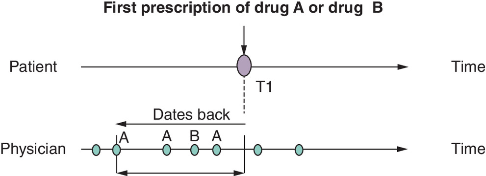
The proportional PPP is the number of certain treatment (X = 1) divided by the number of all prescriptions made by this physician (Equation 3).
(Equation 3)
Equation 3. Calculation of the proportional PPP.
All analysis is done in R studio using R version 3.6.1. The R code that generates the simulated datasets and the regression models can be found in the appendix.
Results
Percent bias
Figure 2 presents the percent bias of the 2SLS and OLS in moderate and small sample sizes. OLS is subject to unmeasured confounding bias (Figure 2). In the case of a lower unmeasured confounding level, the 2SLS is more biased than OLS. The advantage of 2SLS appears after the level of the unmeasured confounding increases. The sample size does not influence the percent bias in general.
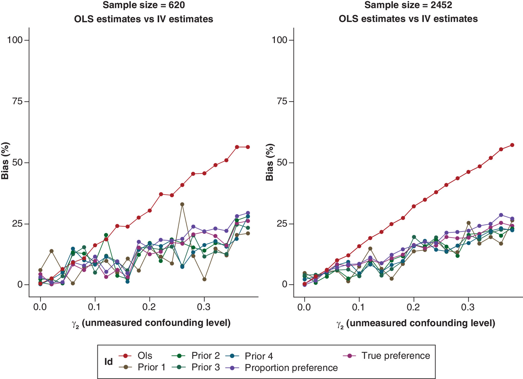
Figure 2. Percent bias of estimates from two-stage least squares and ordinary least squares.
IV: Instrumental variable; OLS: Ordinary least squares.
The coverage rate shows that that the 2SLS covers nominal 95% while the coverage rate of OLS drops dramatically in both sample sizes (Figure 3). This can be explained by Equation 4 where the difference between the variances of OLS estimates and variances of IV estimates is defined by the value of the correlation between the treatment and the IV ( ) [11]. The value of correlation between the treatment and IV are no larger than 1 which make the variance of IV larger than that of the OLS.
(Equation 4)
Equation 4. Variance of IV estimate (2SLS) and OLS estimate. : The residual variance of the outcome after adjusting the treatment (X); : The variance of the treatment; : The correlation between the treatment (X) and the instrumental variable (Z).
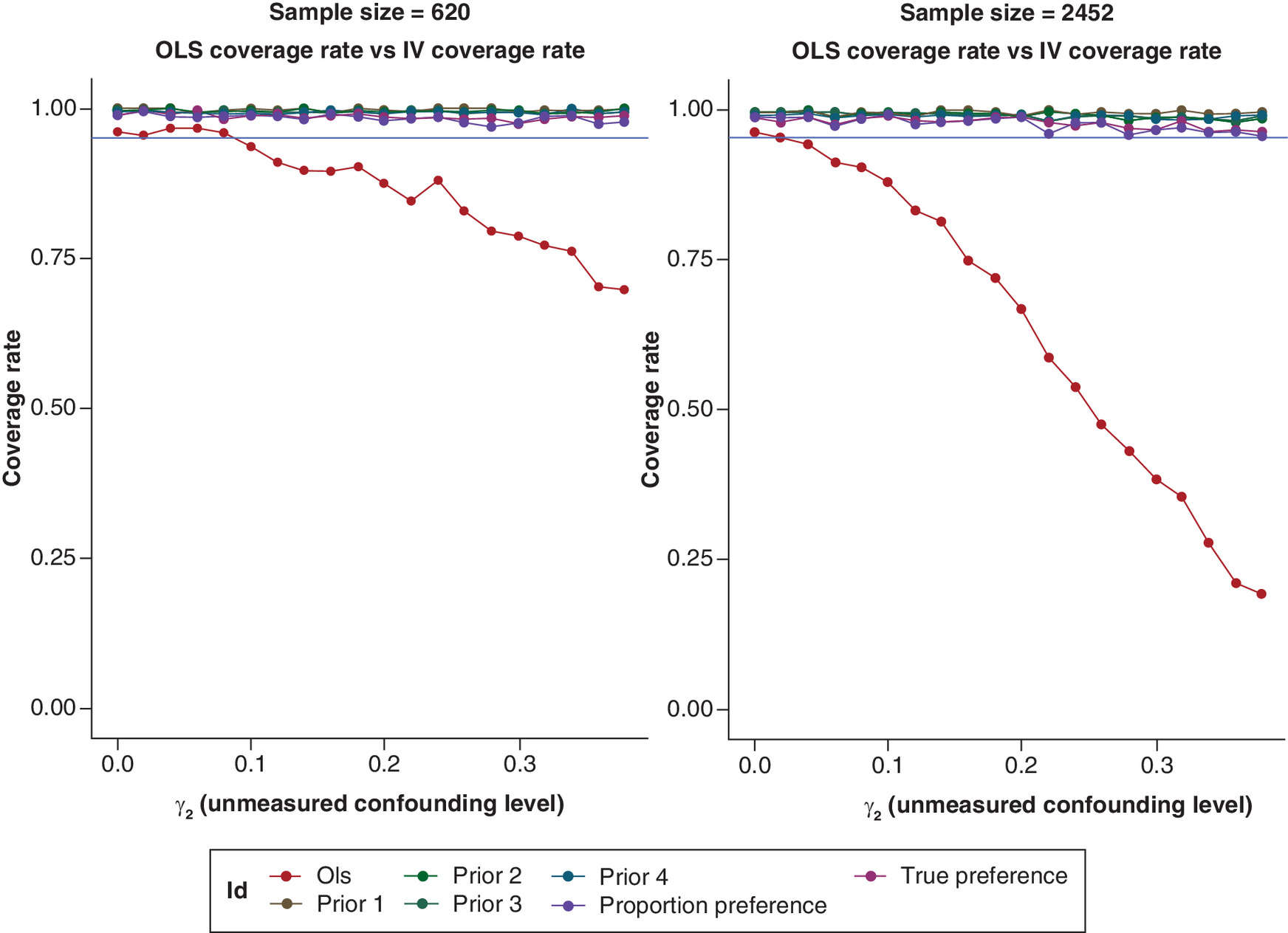
Figure 3. Coverage rate across 1000-times simulation.
The blue intercept line represents the nominal 95%.
IV: Instrumental variable; OLS: Ordinary least squares.
Coverage rate
The strength of the IV increases, and the p value of the 2SLS estimate decreases, as the number of previous prescriptions used in the PPP construction increases (Figure 4). The level of unmeasured confounding does not influence these results. However, the strength of IV decreases noticeably when the sample size decreases. The relation between the F-statistics, sample size and the correlation between the treatment and the IV is shown in Equation 5. The does not change much in these two cases (around 0.14 to 0.15) indicating that the strength of the association between the exposure and instruments does change. Rather, it is the sample size that decreases the F-statistics and makes the IV weaker [11]. The p values of 2SLS estimates in n = 620 sample are consistently larger than that of n = 2452 which means the statistical power of 2SLS is limited by the sample size.
(Equation 5)
Equation 5. : The variance of the treatment; : The correlation between the treatment (X) and the instrumental variable (Z).
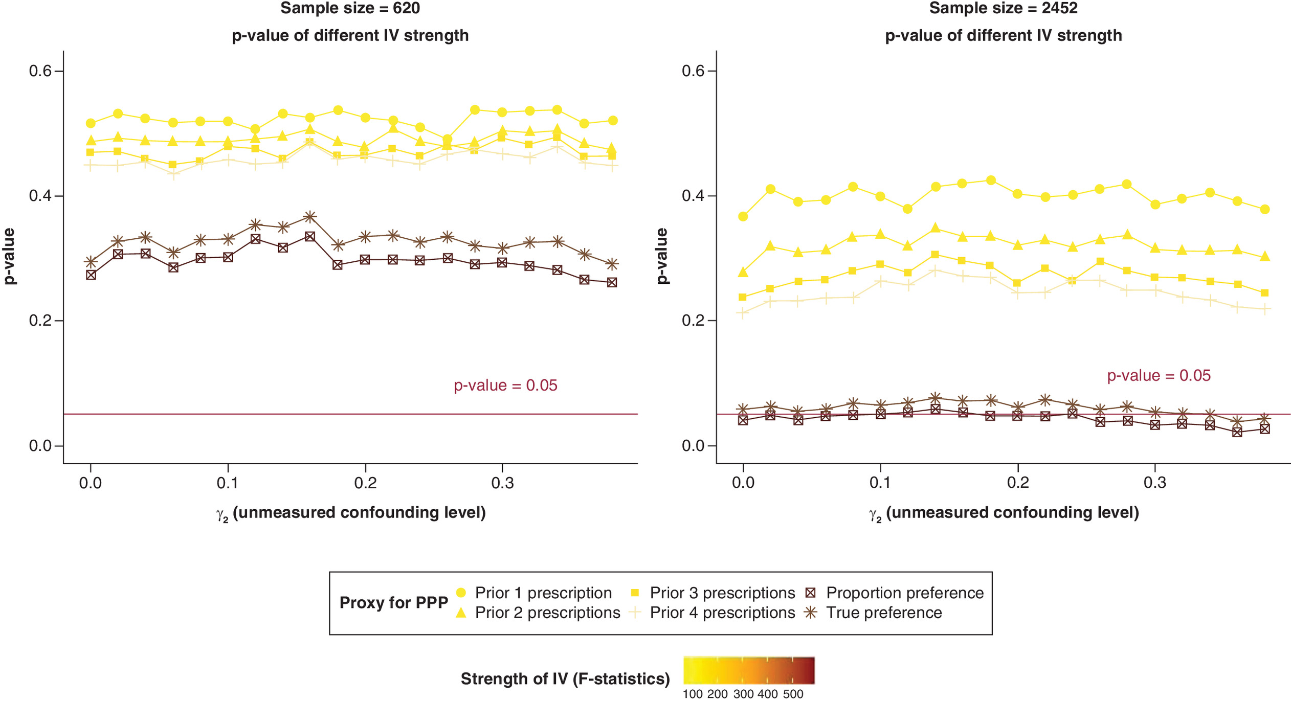
Figure 4. P-values of ordinary least squares estimates and two-stage least squares estimates.
IV: Instrumental variable; PPP: Physician's prescribing preference.
p value of the OLS estimates & 2SLS estimates
As an IV, the true preference (PPP in the model [1]) also shows a strong ability to reduce the unmeasured confounding bias. The F-statistics of true preference reaches 500 which is much higher than all proxies mentioned above (Supplementary Figure 9) which align with the finding from Ionescu-Ittu et al. [9] that the true preference has the smallest variance. The p values for 2SLS estimates are close to conventional statistical significance (p < 0.05). The bias-variance trade-off for IV methods also exist for the ‘true preference’ but not as critical as for the proxy PPP indicating stronger instrument reduces the variance of instrumental variable estimates [12]. The results from the proportion IV indicates that the proportion preference that accounting for whole prescribing history is the strongest IV among these proxies. It is associated with the smallest p value which leads to the 2SLS estimates having small p values.
Confidence interval of OLS estimates & 2SLS estimates
As summarized in Figure 5, 95% confidence intervals of IV estimates narrow as the strength of instruments increases (from prior 1 prescription to the proportional preference). As discussed above, the 95% confidence intervals of OLS estimates are narrower than for 2SLS, and this is also shown in Figure 4. It can also be seen that the OLS estimates are severely biased when the unmeasured confounder covariate parameter ) is set at a high level. Although the IV estimates are generally less precise, it is feasible when the IV is strong enough that an IV estimate can achieve statistical significance while at the same time reducing the influence of unmeasured confounding bias.
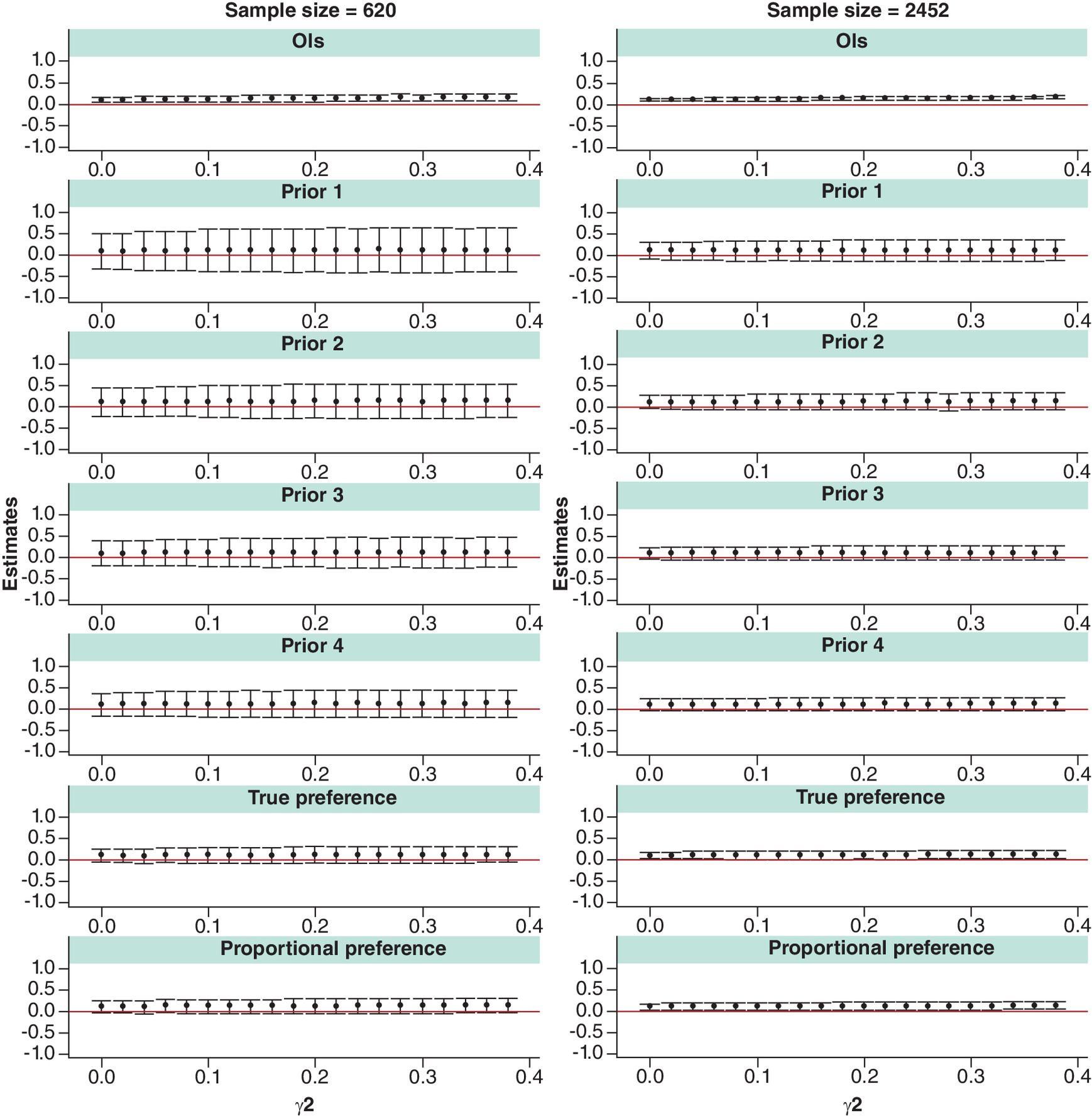
Figure 5. 95% confidence intervals of ordinary least squares and 2SLS estimates.
95% CIs are calculated using cluster robust standard errors. The red line represents the null hypothesis.
OLS: Ordinary least squares.
Discussion
The sample size limits the performance of IVs [7,11]. A straightforward explanation for this is that smaller sample sizes make it harder for the IV to meet the relevance assumption. In real-life CERs, sample sizes are often large enough which can avoid such pitfalls, but when the outcome of interest is rare leading to rare records of medical treatment, or a drug has only recently become available, the corresponding CERs will have smaller sample sizes. This simulation aimed to test the performance PPP IV on the different level of unmeasured confounding level and generate supporting evidence that the PPP IV can perform well in reducing bias in studies of moderate or small sample sizes.
Our results show that 2SLS does reduce the unmeasured confounding to a considerable extent compared with conventional analyses even in a small sample size. At the same time, the standard deviation of 2SLS estimates is generally many times larger than OLS and the confidence interval wide and crossing the null hypothesis. However, if the instrumental variable is strong enough, 2SLS estimates could be statistically significant. In terms of reducing bias, the sample size is not the determinant as it does not impact percent bias. Nevertheless, the sample size does limit the statistical power. In a smaller sample size, the difference of percent bias from 2SLS and OLS can still be an indicator to see if an unmeasured confounding is a major problem although the weak statistical power makes the 2SLS estimate less useful.
The results of this simulation study show that using PPP as an IV is effective at minimizing bias caused by unmeasured confounding relative to only adjusting for measured confounding in CER. The PPP is a latent variable that cannot be measured directly using routinely collected data [1]. Our results show that increasing the number of previous prescriptions used in constructing the PPP leads to power gains which could be particularly important for studies with small or moderate sample sizes. It is worth noting that using PPP with only one previous prescription is a popular strategy in the applied literature. According to our results, prior 2, prior 3, prior 4 and the proportion IV performs better than prior one since the IV strength increases as we account for longer prescription history. It is worth pointing out that by using a larger history in calculating PPP, this implicitly assumes that a physician's preference does not change over time. This can be empirically tested using study data.
Baiocchi and colleagues suggest that researchers should consider the necessity for using IV method to account for unmeasured confounding. If the unmeasured confounding is small, IV methods may not be necessary [13]. We support this conclusion with our simulation results. According to the figures, it is quite noticeable that there a threshold where the percent bias of conventional methods become larger than that of IV methods. If we conduct IV methods at those points, the IV estimates may not be reliable.
The limitation of this study mainly rests on the simplicity of the design. By moderate sample size, we used approximately 2500 which is derived from a research study the authors led on investigating prescribing for alcohol dependence in Scotland. Also, we reviewed the sample sizes that in the current CERs papers that focus on the PPP IV and found that most of them are above 10,000. We did not consider survival analysis including censored outcomes [14] or non-linear two-stage approaches, like two-stage predictor substitution and two-stage residual inclusion, in the simulation design. Finally, we need to emphasize that an essential limitation of studying the time-based proxies for IVs is that the time cannot be truly simulated as all data generated at the same time. The prior 1, 2, 3, 4 prescription proxy estimates are based on real time in applied studies. Strictly speaking, this simulation demonstrates valid proxies for PPP IV, rather than the ‘true’ prior 1, 2, 3, 4 prescriptions as proxies.
Conclusion
Using PPP as an IV for CER is less biased than conventional approaches and can achieve adequate statistical power in smaller sample sizes if the IV strength is high enough. If it can be assumed that a physician's prescribing preference does not change over time, we recommend constructing PPP using entire prescribing history to gain power.
Summary points
•
By utilizing physician's prescribing preference as instrumental variable (IV), 2SLS is less likely to be affected by the unmeasured confounding than ordinary least squares (OLS).
•
Two-stage least squares (2SLS) performs less biased in the case of binary outcome, and binary treatment than OLS.
•
The estimates from 2SLS are less precise than that from OLS.
•
Sample sizes do not directly associate with the level of percent bias of 2SLS.
•
Smaller sample size makes 2SLS estimates less precise.
•
Proxies of physician's prescribing preference IV that consider longer prescribing history serves as stronger IVs.
•
Stronger IV is recommended for the studies with smaller sample size.
Author contributions
L Zhang simulated the data, analyzed the results and drafted the manuscript. J Lewsey and DA McAllister are two supervisors of L Zhang. They revised the draft. And all authors approved the final manuscript.
Acknowledgments
Abstract of this work has been presented at the 13th Asian Conference on Pharmacoepidemiology (ACPE 2021). Record can be found on the website: https://www.asianpharmacoepi.org/wp-content/uploads/2022/12/ACPE13-ePoster-abstracts.pdf.
Financial disclosure
The authors have no financial involvement with any organization or entity with a financial interest in or financial conflict with the subject matter or materials discussed in the manuscript. This includes employment, consultancies, honoraria, stock ownership or options, expert testimony, grants or patents received or pending, or royalties.
Competing interests disclosure
The authors have no competing interests or relevant affiliations with anyorganization or entity with the subject matter or materials discussed in the manuscript. This includes employment, consultancies, honoraria, stock ownership or options, expert testimony, grants or patents received or pending, or royalties.
Writing disclosure
No writing assistance was utilized in the production of this manuscript.
Open access
This work is licensed under the Attribution-NonCommercial-NoDerivatives 4.0 Unported License. To view a copy of this license, visit https://creativecommons.org/licenses/by-nc-nd/4.0/
Supplementary Material
File (supplementary material.docx)
- Download
- 558.38 KB
References
1.
Brookhart MA, Schneeweiss S. Preference-based instrumental variable methods for the estimation of treatment effects: assessing validity and interpreting results. Int. J. Biostat. 3(1), Article 14 (2007).
2.
Kuo YF, Montie JE, Shahinian VB. Reducing bias in the assessment of treatment effectiveness: androgen deprivation therapy for prostate cancer. Med. Care 50(5), 374–380 (2012).
3.
Davies NM, Taylor AE, Taylor GM et al. Varenicline versus nicotine replacement therapy for long-term smoking cessation: an observational study using the Clinical Practice Research Datalink. Health Technol. Assess. 24(9), 1–46 (2020).
4.
Kollhorst B, Abrahamowicz M, Pigeot I. The proportion of all previous patients was a potential instrument for patients' actual prescriptions of nonsteroidal anti-inflammatory drugs. J. Clin. Epidemiol. 69, 96–106 (2016).
5.
Taylor GMJ, Taylor AE, Thomas KH et al. The effectiveness of varenicline versus nicotine replacement therapy on long-term smoking cessation in primary care: a prospective cohort study of electronic medical records. Int. J. Epidemiol. 46(6), 1948–1957 (2017).
6.
Nelson RE, Nebeker JR, Hayden C, Reimer L, Kone K, LaFleur J. Comparing adherence to two different HIV antiretroviral regimens: an instrumental variable analysis. AIDS Behav. 17(1), 160–167 (2013).
7.
Boef AG, Dekkers OM, Vandenbroucke JP, le Cessie S. Sample size importantly limits the usefulness of instrumental variable methods, depending on instrument strength and level of confounding. J. Clin. Epidemiol. 67(11), 1258–1264 (2014).
8.
Zhang Z, Uddin MJ, Cheng J, Huang T. Instrumental variable analysis in the presence of unmeasured confounding. Ann. Transl. Med. 6(10), 182 (2018).
9.
Ionescu-Ittu R, Delaney JA, Abrahamowicz M. Bias-variance trade-off in pharmacoepidemiological studies using physician-preference-based instrumental variables: a simulation study. Pharmacoepidemiol. Drug Saf. 18(7), 562–571 (2009).
10.
Davies NM, Gunnell D, Thomas KH, Metcalfe C, Windmeijer F, Martin RM. Physicians' prescribing preferences were a potential instrument for patients' actual prescriptions of antidepressants. J. Clin. Epidemiol. 66(12), 1386–1396 (2013).
11.
Martens EP, Pestman WR, de Boer A, Belitser SV, Klungel OH. Instrumental variables: application and limitations. Epidemiology 17(3), 260–267 (2006).
12.
Ionescu-Ittu R, Abrahamowicz M, Pilote L. Treatment effect estimates varied depending on the definition of the provider prescribing preference-based instrumental variables. J. Clin. Epidemiol. 65(2), 155–162 (2012).
13.
Baiocchi M, Cheng J, Small DS. Instrumental variable methods for causal inference. Stat. Med. 33(13), 2297–2340 (2014).
14.
Tchetgen Tchetgen EJ, Walter S, Vansteelandt S, Martinussen T, Glymour M. Instrumental variable estimation in a survival context. Epidemiology 26(3), 402–410 (2015).
Information & Authors
Information
Published In
Copyright
© 2024 The authors. This work is licensed under the Attribution-NonCommercial-NoDerivatives 4.0 Unported License
History
Received: 27 March 2023
Accepted: 18 March 2024
Published online: 3 April 2024
Keywords:
Topics
Authors
Metrics & Citations
Metrics
Article Usage
Article usage data only available from February 2023. Historical article usage data, showing the number of article downloads, is available upon request.
Citations
How to Cite
Assessing the performance of physician's prescribing preference as an instrumental variable in comparative effectiveness research with moderate and small sample sizes: a simulation study. (2024) Journal of Comparative Effectiveness Research. DOI: 10.57264/cer-2023-0044
Export citation
Select the citation format you wish to export for this article or chapter.