Application and comparison of generalized propensity score matching versus pairwise propensity score matching
Abstract
Aim: A comparison of conventional pairwise propensity score matching (PSM) and generalized PSM method was applied to the comparative effectiveness of multiple treatment options for lung cancer. Materials & methods: Deidentified data were analyzed. Covariate balances between compared treatments were assessed before and after PSM. Cox proportional hazards regression compared overall survival after PSM. Results & conclusion: The generalized PSM analyses were able to retain 61.2% of patients, while the conventional PSM analyses were able to match from 24.1 to 77.1% of patients from each treatment comparison. The generalized PSM achieved statistical significance (p < 0.05) in 8/10 comparisons, whereas conventional pairwise PSM achieved 1/10. The noted differences arose from different matched patient samples and the size of the samples.
Increasingly, researchers are using big data to enhance their ability to understand how drugs, procedures or other interventions perform in nonexperimental, real-world conditions (e.g., outside of a controlled research setting). Big data networks provide the ability to conduct research in a timely and less costly manner than a prospective clinical trial. However, with the lack of randomization, there is a risk that the clinical and demographic factors that led to the choice of the treatment may have an influence on the outcome rather than the treatment itself. Therefore, methods of bias control have been applied to comparative effectiveness and outcomes research to account for and control the bias resulting from differences in patient characteristics between treatment groups in a nonrandomized, real-world setting.
One of the most frequently used methods is propensity score matching (PSM), which is used to balance a set of predefined baseline covariates between treatment groups [1]. PSM is used to balance groups for observed factors that influence treatment choice by determining the likelihood that a patient is treated based on a logistic regression on available covariates. However, it is influenced by nonrandom loss of patients due to the lack of matching, thus reducing sample size and generalizability [2]. Two common algorithms for matching include the greedy matching and the optimal matching. The optimal matching minimizes the total difference in propensity scores (PS) between matched pairs of patients [3]. The most commonly used method for formation of matched pairs is greedy matching using calipers of a specified width [3], where treated patients are individually selected at random and matched to the untreated neighbor with the closest PS, but no more distant than the specified caliper difference. In the process of matching, however, some patients are excluded and the population becomes less generalizable, statistical power is reduced and results are therefore based on a selected subpopulation that may change the outcome assessment [4]. In essence, by increasing the internal validity by matching, the external validity may be reduced by the reduction in sample size through matching on covariates, and these trade-offs must be evaluated by the researcher to ensure the correct balance between internal and external generalizability is met.
To complicate matters, when there are more than two cohorts of interest, as is common in real-world settings that involve multiple treatment options, PSM becomes more complex. Rassen et al. [5] demonstrate how to match patients simultaneously across three cohorts using 1:1:1 matching while noting the implementation complexities of moving to a higher number of groups. Overall, much of the work for the two cohort situations has not been extended to the multicohort case. While multiple cohort comparisons can be performed using conventional pairwise PSM when there are more than two cohorts, these may produce inconsistent or controversial results due to a lack of a common region of support from the samples of matched patients across comparisons and reduced sample sizes. That is, the matched sample for the comparison of Cohort A versus Cohort B may differ substantially from the matched sample for the comparison of Cohort A versus Cohort C. So, the outcomes from a single Cohort (e.g., Cohort A) may be different in each pairwise comparison because the patients in the A versus C comparison may be those patients most unlikely to receive B. With a multiple pairwise approach, it is theoretically possible to have Cohort A better than Cohort B, Cohort B better than Cohort C, and Cohort C better than Cohort A.
To overcome the limitations of the conventional pairwise PSM and comparison in settings of multiple treatment comparisons, Yang et al. [6] have proposed a novel generalized PSM method based on the work by Rosenbaum and Rubin [1] that instead of matching patients via covariate-based PSs across multiple treatment options, leverage the probability of receiving a treatment to estimate the counterfactual outcomes of each treatment for each patient. Thus, one is able to retain a large sample size or a common support across cohorts in the settings of multiple (>2) cohorts.
The need for appropriate matching in nonrandomized data is evident when studying a disease such as lung cancer. Lung cancer is the most common cancer and the most common cause of death from cancer worldwide. Non-small-cell lung cancer (NSCLC) is the most common form of lung cancer; approximately half of all patients with NSCLC who receive chemotherapy will go on to receive additional treatment due to disease progression or recurrence [8,9]. In the postprogression setting, multiple treatment options are available, thus there is great treatment heterogeneity [10]. Given the increasing need for comparisons of more than two treatment comparisons in comparative effectiveness research, this study was designed to apply and compare conventional pairwise PSM and Yang et al.'s generalized PSM method of bias adjustment to the evaluation of comparative effectiveness of multiple NSCLC treatment options in the post-first progression setting. This population and setting were selected for this applied study of generalized PSM because of the large sample size, multiple treatment options used in routine clinical practice and the practical need to better identify optimal methods to evaluate treatment alternatives. It was hypothesized that the generalized PSM methods would identify a common support, retain a larger sample size and overcome the limitations of conventional pairwise PSM in the case of multiple treatment comparisons.
Materials & methods
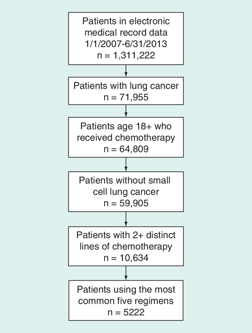
IMS Health Oncology electronic medical record (EMR) data were used for this retrospective cohort study. These EMR data are populated from medium and large community-based oncology practices across the USA. The EMR system from these practices captures detailed, patient-level clinical data that are then deidentified and made available for research purposes. The IMS database through December 2014 includes 1,311,222 individuals visiting medical oncologists and hematologists, of whom approximately 870,000 have a cancer diagnosis, representing data collected from more than 1000 oncologists treating patients from all 50 states.
The EMR data from 1 January 2007 through 31 December 2014 were used for analysis. Eligible patients within this time frame were those who visited a participating oncology clinic and had an initial International Classification of Diseases, Ninth Revision, Clinical Modification (ICD-9-CM) diagnosis of 162.2–162.9 (lung cancer) between 1 January 2007 and 30 June 2013 (to allow for up to 18 months or more of follow-up). Patients were required to be 18 years or older at the time of the first eligible ICD-9 code and were required to have received at least two distinct lines of therapy from the time of index diagnosis to the end of the database. Patients with evidence of small-cell carcinoma were excluded.
Second-line therapy was defined as any new subsequent anticancer systemic treatment introduced more than 28 days after initial anticancer systemic therapy or reintroduction of the initial systemic therapy after a gap of 42 days or more, regardless of the reason for the initiation of a new line of treatment. Overall survival (OS) was defined as the time from the second line of therapy treatment start date to the date of death. Death was assumed to occur on the 15th of the indicated month in order to minimize the error due to death month and year are only available in the database due to requirements of deidentified datasets. A subset of patients has linked data in IMS to the date of death from an Experian database. Due to the limited availability of reported death dates (12.8%), a proxy death date using the last visit in the EMR data was determined for each study patient. The last EMR visit record was assumed to be the date of death if a sufficient period had elapsed between the last visit and the end of the IMS data. A sufficient period of time was defined as at least twice the average visit interval in the 3 months (91 days) prior to last visit. This approach to define a proxy death date has been validated and applied to multiple research projects involving IMS and other observational real-world databases [11–14]. Patients alive at the end of the IMS data (e.g., December 2014) were censored at the end of the IMS data. Additionally, patients who did not have a sufficient period of time between last visit and the end of the data were censored at the last visit. A correlation analysis was performed between the Experian reported death dates and the proxy death dates.
Descriptive statistics were used to summarize patient demographic and clinical characteristics. No imputation was made for missing data. Missing data were summarized as a category for each variable of interest [15]. A patient with partial data was included in the summary whenever data are available. To maximize the use of data information, missing data were included as its own category, ‘Unknown/Missing’, in the PS estimation.
Unadjusted survival analysis
The Kaplan–Meier method was used to estimate median OS and the 95% CI by second-line treatment.
Conventional pairwise PS-matched survival analyses
A binomial logistic regression model (SAS PROC LOGISTIC) was used to calculate PSs for each pair of second-line treatment options using available demographic and baseline clinical characteristics of age, gender, race, region, Eastern Cooperative Oncology Group performance status [16], cancer stage at diagnosis, histology, facility type (academic vs community center) and year of index diagnosis. All these variables were considered to have potential impact on treatment selection and outcomes of the treatment. In the logistic regression model, the binary treatment (1 vs 2) was the dependent variable and the demographic and baseline clinical characteristics were the independent variables. A greedy PSM without replacement [17] was performed on the logit of the PS against the caliper of 0.2-times the pooled standard deviation of the logit of the PSs [18].
In the greedy matching, a subject from Cohort 1 is first selected at random. The subject from Cohort 2 whose PS is closest to that of this randomly selected subject from Cohort 1 is chosen for matching to this subject from Cohort 1. This process is then repeated until subjects from Cohort 2 have been matched to all subjects from Cohort 1 or until one has exhausted the list of subjects from Cohort 1 for whom a matched subject from Cohort 2 can be found. This process is called greedy because at each step in the process, the nearest subject from Cohort 2 is selected for matching to the given subject from Cohort 1, even if that subject from Cohort 2 would better serve as a match for a subsequent subject from Cohort 1.
Balance between the compared cohorts (e.g., treatment groups) was assessed by using absolute standardized differences (d) in covariates before and after matching, respectively [3]. For a continuous covariate, the standardized difference is defined as:
where  and
and  denote the sample mean of the covariate for patients in Cohort 1 and Cohort 2, respectively, whereas
  and
and  denote the sample variance of the covariate for patients in Cohort 1 and Cohort 2, respectively. For dichotomous variables, the standardized difference is defined as:
where  and
and  denote the prevalence of the dichotomous variable for patients in Cohort 1 and Cohort 2, respectively [3]. A covariate is considered to be balanced if the absolute value of the standardized difference is less than 0.1 [19].
A Cox proportional hazard regression analysis (SAS PROC PHREG) was conducted on the PS-matched data to compare differences in OS by treatment. Because balance was reached after PSM, the Cox model contained treatment as the only independent variable. Median OS and hazard ratio (HR), 95% CI and log-rank p-values were estimated from the Cox model.
Generalized PS-adjusted survival analyses
Generalized PSs were generated using a multinomial logistic regression model (SAS PROC LOGISTIC) with multiple treatments as nominal-dependent variable. The model incorporated the same demographic and baseline clinical characteristics as the conventional pairwise PSM approach. As a critical step for quality matching [6], a subgroup of patients with improved overlap in the covariate distribution and minimum variance of the covariate space was identified. For the binary treatment case, Crump et al. [20] proposed a method to improve overlapping by dropping patients with low and high PSs. The threshold for dropping patients is based on minimizing the variance of the estimated average treatment effect on the trimmed sample, in other words, choosing covariate space  to minimize the variance
  .
.
where p(w|x) is the PS, σ 2 is the variance of the estimated average treatment effect on the original population.
To implement Yang et al.'s trimming method [6], the following five steps were followed: Define the function g(x) that is the sum of the inverse of the PSs over T-treatment groups for each patient.
Calculate the g(x) value for each patient based on the generalized PSs; Sort the dataset by g(x) values; Define the function hλ, which is a convex function with a global minimum depending on the value of g(x)
which calculates the h(λ) value for each patient; Find the value of λ, one of the g(x), that minimizes h(λ). The minimum must be attained at one of the N values of g(Xi), so simply evaluate the h(λ) value for each patient (N of them) and take the one that minimizes h(λ); and Exclude patients with g(x) > λ.
Methods for imputation of generalized PSM after the above trimming steps
The generalized PSs were calculated again for the identified common cohort. This is necessary because the generalized PSs calculated initially were based on the original study population. The covariate space changed after trimming and the recalculated generalized PSs exactly reflect the covariate space in the trimmed patient population. Generalized PSM with replacement was performed on the common cohort to obtain counterfactual outcomes under each treatment for each patient. In brief, we impute survival outcomes for each patient for each treatment group based on the observed OS outcomes and the generalized PSs. A simple example using an artificial data to show how this would work in practice is presented in Table 1. Consider Patient 1. For this patient, W1 = 1, so that Ŷ1(1) is actually observed. To impute the missing potential outcome Y1(2) for Patient 1 at treatment level 2 with PS = 0.80, look among the three patients with Wi = 2 for the patient closest in terms of the generalized PS at treatment level 2. That leads to match Patient 7 with PS = 0.79, so that the imputed value for Y1(2) is equal to Ŷ1(2) = Y7 obs = 96. To impute Y1(3) for Patient 1 at treatment level 3 with PS = 0.09, look among the two patients with Wi = 3 for the closest patient in terms of the generalized PS at treatment level 3. That leads to match Patient 8 with PS = 0.10, so that Ŷ1 (3) = Y8 obs = 130. Follow the same steps to impute counterfactual outcomes for each patient at each treatment level. Note that with such a small sample in this simple example, many of the matches are of poor quality. Therefore, the trimming process as described above is an important and necessary step to improve the quality of matching (nearest matching) and counterfactual outcome imputation.
| Patient | Treatment | Observed and potential outcomes [1] | Generalized propensity score | Observed outcomes | Imputed counterfactual outcomes | ||||||
|---|---|---|---|---|---|---|---|---|---|---|---|
| i | Wi | Yi (1) | Yi (2) | Yi (3) | p(1|Xi) | p(2|Xi) | p(3|Xi) | Yi obs | Ŷi (1) | Ŷi (2) | Ŷi (3) |
| 1 | 1 | 102 | ? | ? | 0.11 | 0.80 | 0.09 | 102 | 102 | 96 | 130 |
| 2 | 1 | 105 | ? | ? | 0.34 | 0.35 | 0.31 | 105 | 105 | 94 | 80 |
| 3 | 1 | 120 | ? | ? | 0.20 | 0.50 | 0.30 | 120 | 120 | 96 | 80 |
| 4 | 1 | 108 | ? | ? | 0.19 | 0.31 | 0.50 | 108 | 108 | 94 | 80 |
| 5 | 2 | ? | 100 | ? | 0.83 | 0.04 | 0.13 | 100 | 105 | 100 | 130 |
| 6 | 2 | ? | 94 | ? | 0.09 | 0.09 | 0.82 | 94 | 102 | 94 | 80 |
| 7 | 2 | ? | 96 | ? | 0.01 | 0.79 | 0.20 | 96 | 102 | 96 | 130 |
| 8 | 3 | ? | ? | 130 | 0.75 | 0.15 | 0.10 | 130 | 105 | 94 | 130 |
| 9 | 3 | ? | ? | 80 | 0.35 | 0.30 | 0.35 | 80 | 105 | 94 | 80 |
The numbers are the observed outcomes, while the question marks are the outcomes to be imputed, in other words, counterfactual outcomes.
Balance between the compared cohorts was assessed by using absolute standardized differences (d) in covariates before and after pairwise PSM. Following the process of Yang et al. for the generalized PSM, perfect (d = 0) balance is achieved by definition as each patient retains the same covariates for all treatment levels [6]. A Cox proportional hazards regression analysis (SAS PROC PHREG) was conducted on the generalized PS-matched data, as illustrated in right three columns in Table 1, to compare OS outcomes by the five most common treatments in a single model. Because the cohorts were balanced after PSM, the Cox model contained treatment as the only independent variable. Median OS for each treatment and pairwise HR, 95% CI and log-rank p-value were estimated from the Cox model.
Sensitivity analysis
A sensitivity analysis was conducted using bootstrapping to evaluate the OS results from the Cox model. The generalized PS-matched data are an N × T data table, where N is the number of patients in the common cohort and T is the number of treatments, as illustrated in right three columns in Table 1. One thousand bootstrapping samples of the counterfactual OS outcomes were drawn with replacement from the common cohort for each of the five most common treatments using SAS PROC SURVEYSELECT. The median and 95% CI of the median were calculated for each treatment. The p-value is assumed less than 0.05 if the CIs are not overlapping between a pair of treatments in comparison. This analysis was conducted to reconfirm the treatment comparison results from the Cox regression model by using the nonparametric bootstrapping approach.
All analyses were conducted using SAS Version 9.3 statistical software (SAS Institute Inc., NC, USA) at a priori significance level of 0.05. No adjustment for multiple comparisons was made.
Interested readers who use SAS or R may refer to the appendix table – for coding support to conduct generalized PSM. For R users, Yang et al. provided supplementary web appendices for generalized PSM and a simulation study [6]. In their supplementary appendices, the authors also provide mathematical details for inference and show that under mild regularity conditions, the matching estimator based on the generalized PS or the estimated generalized PS is asymptotically normally distributed.
Results
Patients receiving postprogression therapy
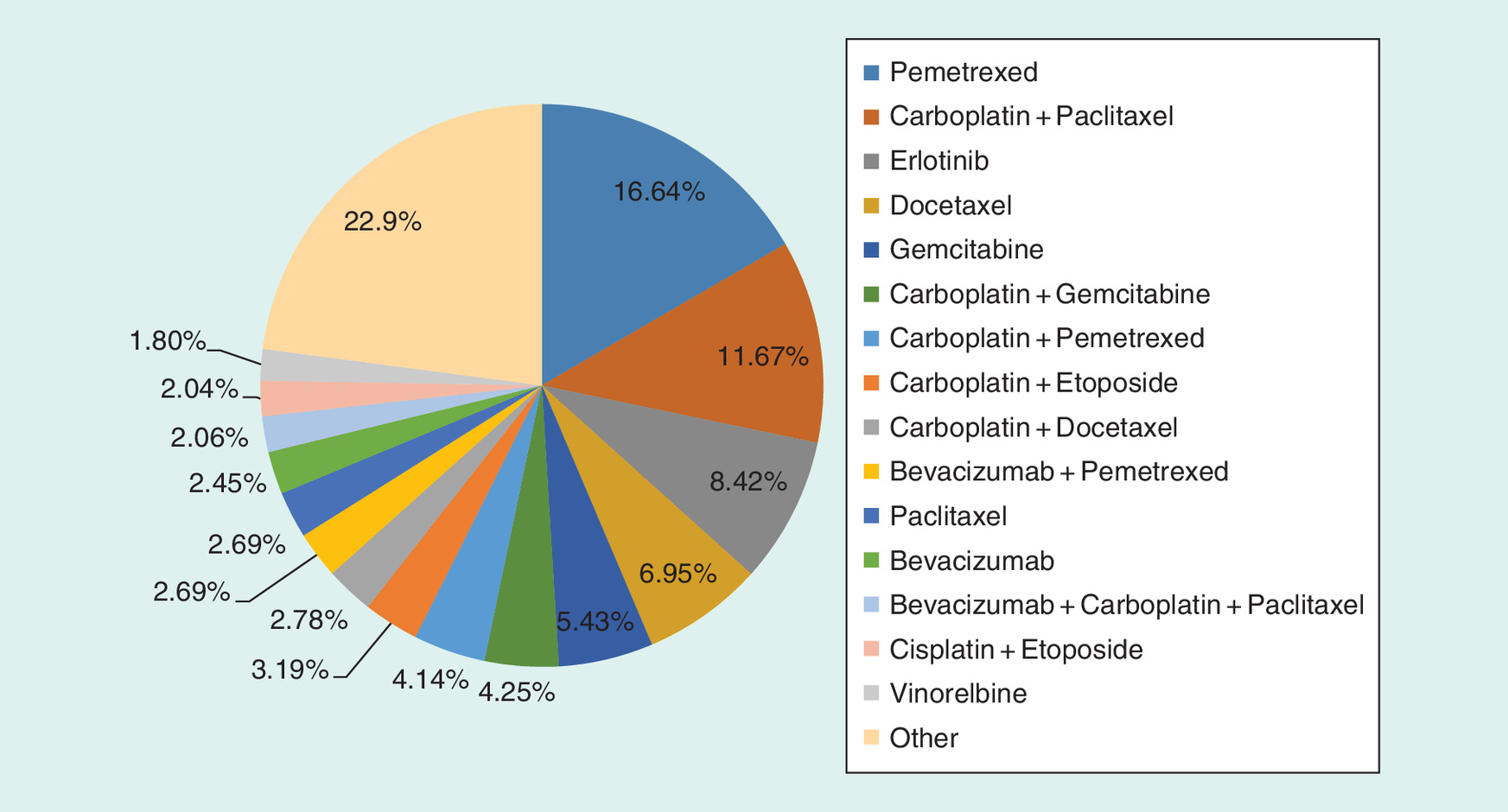
A total of 10,634 patients met all eligibility criteria and were included in this study (Figure 1). The demographic and baseline clinical characteristics of these patients are presented in Table 2. The most common treatments used in this setting (Figure 2) were single-agent pemetrexed (16.6%), followed by carboplatin + paclitaxel (11.7%), single-agent erlotinib (8.4%), single-agent docetaxel (7.0%) and single-agent gemcitabine (5.4%). The five most common treatments account for 49.1% (5222) of the study population and were selected for further effectiveness comparisons to examine the differences in PSM methods. The proxy death date demonstrated a very high correlation (r > 0.99) with the Experian death date; therefore, all results are presented using the proxy date alone.
| Characteristics | Eligible patients (n = 10,634) | Pemetrexed (n = 1770) | Carboplatin + paclitaxel (n = 1241) | Erlotinib (n = 895) | Docetaxel (n = 739) | Gemcitabine (n = 577) |
|---|---|---|---|---|---|---|
| Age at initiation of postprogression therapy | ||||||
| Mean (SD) | 66.4 (9.9) | 66.5 (9.7) | 66.7 (9.6) | 68.3 (9.8) | 65.5 (9.7) | 68.6 (9.5) |
| Median (range) | 67 (18–85) | 67 (36–84) | 68 (41–84) | 70 (33–85) | 66 (34–85) | 69 (38–85) |
| Sex, n (%) | ||||||
| Unknown | 1 (0%) | 1 (0.1%) | 0 (0.0%) | 0 (0.0%) | 0 (0.0%) | 0 (0.0%) |
| Male | 5741 (54%) | 927 (52.4%) | 734 (59.1%) | 439 (49.1%) | 452 (61.2%) | 316 (54.8%) |
| Female | 4892 (46%) | 842 (47.6%) | 507 (40.9%) | 456 (50.9%) | 287 (38.8%) | 261 (45.2%) |
| Race, n (%) | ||||||
| Unknown | 3059 (28.8%) | 587 (33.2%) | 336 (27.1%) | 234 (26.1%) | 210 (28.4%) | 178 (30.8%) |
| African American | 685 (6.4%) | 138 (7.8%) | 70 (5.6%) | 78 (8.7%) | 63 (8.5%) | 45 (7.8%) |
| Asian | 77 (0.7%) | 13 (0.7%) | 5 (0.4%) | 18 (2%) | 2 (0.3%) | 5 (0.9%) |
| Caucasian | 6354 (59.8%) | 967 (54.6%) | 787 (63.4%) | 516 (57.7%) | 438 (59.3%) | 330 (57.2%) |
| Other | 420 (3.9%) | 62 (3.5%) | 38 (3.1%) | 45 (5%) | 24 (3.2%) | 19 (3.3%) |
| Hispanic | 39 (0.4%) | 3 (0.2%) | 5 (0.4%) | 4 (0.4%) | 2 (0.3%) | 0 (0.0%) |
| Disease stage at initial diagnosis, n (%) | ||||||
| Stage unknown | 6369 (59.9%) | 994 (56.2%) | 756 (60.9%) | 498 (55.6%) | 421 (57%) | 313 (54.2%) |
| Stage 0 | 7 (0.1%) | 1 (0.1%) | 3 (0.2%) | 0 (0.0%) | 0 (0.0%) | 0 (0.0%) |
| Stage I | 234 (2.2%) | 37 (2.1%) | 31 (2.5%) | 27 (3%) | 12 (1.6%) | 7 (1.2%) |
| Stage II | 339 (3.2%) | 44 (2.5%) | 64 (5.2%) | 28 (3.1%) | 22 (3%) | 25 (4.3%) |
| Stage III | 1483 (13.9%) | 230 (13%) | 226 (18.2%) | 126 (14.1%) | 107 (14.5%) | 79 (13.7%) |
| Stage IV | 2202 (20.7%) | 464 (26.2%) | 161 (13%) | 216 (24.1%) | 177 (24%) | 153 (26.5%) |
| ECOG PS score at initiation of postprogression therapy, n (%) | ||||||
| Unknown | 6780 (63.8%) | 1119 (63.2%) | 812 (65.4%) | 541 (60.4%) | 483 (65.4%) | 358 (62%) |
| PS = 0 | 530 (5%) | 115 (6.5%) | 57 (4.6%) | 48 (5.4%) | 35 (4.7%) | 27 (4.7%) |
| PS = 1 | 1799 (16.9%) | 318 (18%) | 204 (16.4%) | 149 (16.6%) | 125 (16.9%) | 95 (16.5%) |
| PS = 2 | 1158 (10.9%) | 164 (9.3%) | 137 (11%) | 122 (13.6%) | 71 (9.6%) | 74 (12.8%) |
| PS = 3 | 343 (3.2%) | 53 (3%) | 28 (2.3%) | 33 (3.7%) | 21 (2.8%) | 20 (3.5%) |
| PS = 4 | 24 (0.2%) | 1 (0.1%) | 3 (0.2%) | 2 (0.2%) | 4 (0.5%) | 3 (0.5%) |
| Histology, n (%) | ||||||
| Squamous | 736 (6.9%) | 0 (0.0%) | 152 (12.2%) | 56 (6.3%) | 68 (9.2%) | 64 (11.1%) |
| Nonsquamous | 7181 (67.5%) | 1770 (100%) | 645 (52%) | 511 (57.1%) | 446 (60.4%) | 283 (49%) |
| Unknown | 2717 (25.6%) | 0 (0.0%) | 444 (35.8%) | 328 (36.6%) | 225 (30.4%) | 230 (39.9%) |
| Practice setting, n (%) | ||||||
| Other | 846 (8%) | 184 (10.4%) | 79 (6.4%) | 4 (0.4%) | 48 (6.5%) | 46 (8%) |
| Community-based | 8898 (83.7%) | 1446 (81.7%) | 1019 (82.1%) | 882 (98.5%) | 630 (85.3%) | 503 (87.2%) |
| Hospital-based | 890 (8.4%) | 140 (7.9%) | 143 (11.5%) | 9 (1%) | 61 (8.3%) | 28 (4.9%) |
ECOG: Eastern Cooperative Oncology Group; PS: Performance status; SD: Standard deviation.
Resultant sample sizes by the PS method
Using conventional pairwise PSM, ten comparator treatment matches were performed with different levels of successful matches (Table 3). The matching rate was calculated as the number of matched patients divided by the total number of patients in the compared treatment groups. The lowest percent of matching was 24.1%; the highest is 77.1%, both demonstrating good matching characteristics. When applying the generalized PSM (Table 4), a common cohort was identified by trimming patients with extreme PS values [6], resulting in 61.2% retention. The generalized PSM retained 61.2% (42.5–87.7%) of the patient sample from the five treatments.
| Treatments | Matched treatments (conventional pairwise propensity score matching) | ||||
|---|---|---|---|---|---|
| Pemetrexed (n = 1770) | Carboplatin + paclitaxel (n = 1241) | Erlotinib (n = 895) | Docetaxel (n = 739) | Gemcitabine (n = 577) | |
| Pemetrexed (n = 1770) | – | 42.7% | 38.3% | 35.5% | 24.1% |
| Carboplatin + paclitaxel (n = 1241) | 643 | – | 66.6% | 71.2% | 59.0% |
| Erlotinib (n = 895) | 511 | 711 | – | 70.3% | 65.1% |
| Docetaxel (n = 739) | 445 | 705 | 574 | – | 77.1% |
| Gemcitabine (n = 577) | 283 | 536 | 479 | 507 | – |
The matching percent was calculated as the number of matched patients divided by the total number of patients in the compared treatment groups, for example, the matching percent for pemetrexed versus carboplatin + paclitaxel is calculated as 643 × 2/(1770 + 1241) = 42.7%. The matching percent can also be calculated as the number of matched pairs divided by the number of patients in the smaller treatment group in comparison, for example, the matching percent for pemetrexed versus carboplatin + paclitaxel is calculated as 643/1241 = 51.8% (data not shown in the table).
| Treatment | Total number of patients | Trimmed number of patients | Remaining number (%) of patients |
|---|---|---|---|
| Overall | 5222 | 2027 | 3195 (61.18) |
| Pemetrexed | 1770 | 217 | 1553 (87.74) |
| Carboplatin + paclitaxel | 1241 | 702 | 539 (43.43) |
| Erlotinib | 895 | 430 | 465 (51.96) |
| Docetaxel | 739 | 346 | 393 (53.18) |
| Gemcitabine | 577 | 332 | 245 (42.46) |
Binary PS-adjusted survival analyses
Balances in the baseline covariates between treatments were achieved after pairwise PSM (Supplementary Figures). The absolute standardized differences were acceptable (d < 0.1) in general, with some exceptions at certain categorical levels. When comparing between treatment options, one of ten (10%) pairwise comparisons showed statistically significant differences in OS outcomes using the conventional pairwise PSM method (Table 5).
| Comparison pair | Median OS HR (95% CI), p-value | ||
|---|---|---|---|
| Conventional propensity score matching† | Generalized propensity score‡ | Bootstrapping§ | |
| Pemetrexed vs carboplatin + paclitaxel | 6.48 vs 8.55 1.07 (0.83, 1.39), p = 0.591 | 7.20 vs 8.45 1.02 (0.98, 1.07), p = 0.290 | 7.04 (6.84, 7.46) vs 8.12 (7.78, 8.45), NS |
| Pemetrexed vs gemcitabine | 6.94 vs 5.65 0.63 (0.4, 0.99), p = 0.046 | 7.20 vs 5.59 0.79 (0.76, 0.83), p < 0.0001 | 7.04 (6.84, 7.46) vs 5.56 (5.49, 5.59), p < 0.05 |
| Pemetrexed vs erlotinib | 7.89 vs 9.11 1.2 (0.9, 1.6), p = 0.225 | 7.20 vs 8.94 1.19 (1.14, 1.25), p < 0.0001 | 7.04 (6.84, 7.46) vs 8.55 (8.02, 8.84), p < 0.05 |
| Carboplatin + paclitaxel vs erlotinib | 8.15 vs 9.47 1.37 (0.97, 1.95), p = 0.077 | 8.45 vs 8.94 1.14 (1.1, 1.2), p < 0.0001 | 8.12 (7.78, 8.45) vs 8.55 (8.02, 8.84), p < 0.05 |
| Carboplatin + paclitaxel vs gemcitabine | 8.45 vs 5.62 0.9 (0.62, 1.29), p = 0.556 | 8.45 vs 5.59 0.76 (0.72, 0.79), p < 0.0001 | 8.12 (7.78, 8.45) vs 5.56 (5.49, 5.59), p < 0.05 |
| Erlotinib vs docetaxel | 7.66 vs 6.67 0.74 (0.52, 1.06), p = 0.105 | 8.94 vs 5.95 0.7 (0.67, 0.73), p < 0.0001 | 8.55 (8.02, 8.84) vs 5.82 (5.49, 5.95), p < 0.05 |
| Erlotinib vs gemcitabine | 7.43 vs 5.65 0.71 (0.45, 1.14), p = 0.160 | 8.94 vs 5.59 0.67 (0.64, 0.7), p < 0.0001 | 8.55 (8.02, 8.84) vs 5.56 (5.49, 5.59), p < 0.05 |
| Docetaxel vs pemetrexed | 6.67 vs 6.21 0.92 (0.68, 1.25), p = 0.604 | 5.95 vs 7.20 0.82 (0.78, 0.86), p < 0.0001 | 5.82 (5.49, 5.95) vs 7.04 (6.84, 7.46), p < 0.05 |
| Carboplatin + paclitaxel vs docetaxel | 8.55 vs 6.12 0.89 (0.66, 1.19), p = 0.435 | 8.45 vs 5.95 0.77 (0.74, 0.81), p < 0.0001 | 8.12 (7.78, 8.45) vs 5.82 (5.49, 5.95), p < 0.05 |
| Docetaxel vs gemcitabine | 6.02 vs 5.56 0.77 (0.52, 1.13), p = 0.185 | 5.95 vs 5.59 0.96 (0.92, 1), p = 0.056 | 5.82 (5.49, 5.95) vs 5.56 (5.49, 5.59), NS |
†HR, 95% CI and log-rank p-value were based on a Cox proportional hazards regression model with the compared treatment as the only independent variable. Median OS from start of second-line treatment to death was estimated using the Kaplan–Meier method.
‡HR, 95% CI and log-rank p-value were based on a Cox proportional hazards regression model with the compared treatment as the only independent variable. Median OS from start of second-line treatment to death was estimated using the Kaplan–Meier method.
§Bootstrapping was conducted on the counterfactual OS outcomes imputed using generalized propensity score matching. The median and the CI were obtained from bootstrapping sample size of 1000.
Bold values represent values which are statistically significant.
HR: Hazard ratio; NS: Not significant; OS: Overall survival (in months).
Generalized PS-adjusted survival analyses
Balances in the baseline covariates between compared treatments were achieved after generalized PSM (Supplementary Figures). A satisfactory balance was achieved for both missing and nonmissing categories. The absolute standardized differences were acceptable (d = 0 by definition per Yang et al. [6]). Results by treatment after controlling for demographic and baseline clinical characteristics using generalized PSM are presented in Table 5. When comparing between treatment options, eight of ten (80%) pairwise comparisons showed statistically significant differences.
Sensitivity analysis
Bootstrapping of the counterfactual OS outcomes imputed using generalized PSM confirmed the results from the Cox proportional hazards regression models, with the same eight of ten comparisons remaining statistically significant (Table 5).
Discussion
This study applied and compared different bias control methods, the novel generalized PSM proposed by Yang et al. [6] and conventional pairwise PSM, to a comparative effectiveness research question in a setting of multiple treatment comparisons. The evaluation of findings across methods revealed several key findings for researchers to consider when selecting bias control methods in the conduct of comparative effectiveness research using real-world data. It is important to note there is no ‘gold standard’ method for bias control particularly in the setting of multiple treatment options. The selection among options must be made based on the availability of data and the scientific question and study goals, with an awareness and knowledge of the strengths and limitations of each approach. The generalized PSM may have potential applications in observational studies with multiple treatments, as it was successfully able to retain greater statistical power by maintaining a larger proportion of the original study sample size, and enabled simultaneous comparisons that are more applicable to clinical decision-making without the need to interpret a series of pairwise comparisons. The generalized PSM demonstrated similar median OS estimates to the conventional pairwise PSM with some variation. Importantly, the generalized PSM demonstrated the ability to make simultaneous comparisons across multiple treatments on a common support. In addition, the ability to retain a larger study sample provided greater statistical power to identify statistically significant differences between treatment groups. As with all studies using big data, the investigator must further ensure that the statistical differences are clinically meaningful.
For both the conventional pairwise PSM and the generalized PSM methods, results could have been affected if the underlying assumption of ‘no unmeasured confounding’ was not true. Potential unmeasured confounders, such as medical insurance plan, biomarker and financial status, may affect the choice of treatment and outcome of the treatment. Rarely will a real-world data source contain every variable that could affect outcomes. The researchers conducting the study must ensure missing data are minimized and that no critical variables are absent from the dataset, or other approaches must be taken to address the data gaps (e.g., instrumental variables, imputation of missing data), all of which have their own strengths and weaknesses.
Though the generalized PSM demonstrated the ability to consistently adjust the comparisons across multiple cohorts using a common population of inference, the covariate balance may be overstated. This is because, by definition, the patient retains the same covariates across multiple treatments during the imputation of the counterfactual outcomes. In fact, the generalized PSM is a nearest matching (not exact matching), thus the imputed counterfactual outcomes for a patient could have come from multiple patients with slightly different covariates. Therefore, caution must be taken when using the generalized PSM alone. An alternative balance assessment may be done using the imputed covariates. To do this, we not only impute the counterfactual outcomes but also impute the covariates. Signaled by the fact that eight out of ten comparisons in the generalized PSM versus one out of ten comparisons in the conventional pairwise PSM were statistically significant, we believe, the noted differences arose from different matched patient samples and the size of the samples. We also believe that the variance for comparisons among multiple treatments played an important role. In the imputation of counterfactual outcomes with replacement, some observed outcomes could have been used multiple times, resulting in a decrease in variance.
It is possible that some covariates influencing mortality may differ from those influencing treatment choice. Therefore, controlling for covariate differences at time of treatment choice may not be sufficient. In cases where these variables differ, doubly robust estimators [22] may complement the PSM approach by further applying a stepwise Cox regression model to select significant covariates after PSM. Additionally, further sensitivity analyses could be conducted to investigate the imputation of the counterfactual outcomes, such as applying a caliper in the nearest matching of the generalized PSs to avoid poor matching, allowing multiple matches such as 1:k matches instead of the standard 1:1 match, and using the average of the k-matched outcomes as the counterfactual outcome.
In summary, comparative analyses based on real-world datasets are at risk of confounding biases. Due to the lack of randomization, the factors that contribute to the choice of treatment may also contribute to the differences in outcomes. Therefore, methods must be used in any comparative analyses to balance any potential prognostic factors that may contribute to the outcome of interest to ensure comparability between groups. This study demonstrated many differences in results that are likely due to confounding and the ability of each method to control for the differences between treatment groups. As with all nonrandomized, real-world datasets, it is recommended that comparative analyses be conducted in cases where observational data have very low rates of missing data and include potential confounders relevant to the research question being asked. In this study, some factors were not well represented in the data, such as histology, and imputation was made for histology based on the treatments received to reduce this risk. It is important to note that neither conventional nor generalized PS methods can account for potential events that may occur after the initiation of the treatment being compared (e.g., side effects or time to disease progression). There is a risk that these time-dependent confounders could influence duration of therapy, choice or lack of subsequent therapy, and thereby influence the outcomes being measured in this study. These cannot be controlled for using conventional or generalized PS methods.
This paper is an application and comparison of the existing methods, not intending to improve the methods. Future research should evaluate the balance assessment and variance for the treatment effect using the generalized PSM. These could be done by further analyses of this case study data or similar and a series of simulations.
Conclusion
Despite the limitations of these methods, this study has demonstrated the potential application of the generalized PSM to comparative effectiveness research with multiple comparisons. The retention of more eligible cases from the data provides a greater sample size to detect statistically significant differences and simultaneous comparisons across cohorts on a common support. It is recommended that this method be applied in combination with predefined sensitivity analyses to explore potential biases introduced by the method.
There are various methods available to adjust for potential confounding in nonrandomized, observational comparative effectiveness research.
Commonly used methods, such as conventional propensity score matching, have limitations in analysis of multiple comparisons.
This study compared a novel generalized propensity score method with conventional pairwise propensity score matching.
The generalized propensity score method demonstrated the ability to consistently adjust the comparisons across multiple cohorts using a common population of inference while minimizing loss of patient samples.
Supplementary data
To view the supplementary data that accompany this paper please visit the journal website at: Supplementary Material
Acknowledgements
The research team thank Julie Beyrer, for her support in the study design and manuscript review.
Financial & competing interests disclosure
All the authors are employees of Eli Lilly and Company. The authors have no other relevant affiliations or financial involvement with any organization or entity with a financial interest in or financial conflict with the subject matter or materials discussed in the manuscript apart from those disclosed.
No writing assistance was utilized in the production of this manuscript.
Ethical conduct of research
This study utilized a deidentified dataset, which is not considered human subjects research under the U.S. Code of Federal Regulations. All the authors meet the requirements for authorship as outlined by the International Committee of Medical Journal Editors (ICMJE) Recommendations for the Conduct, Reporting, Editing and Publication of Scholarly Work in Medical Journals (http://www.ICMJE.org). All the authors have reviewed and approved the final manuscript for submission.
Supplementary Material
File (suppl_materials.docx)
- Download
- 766.04 KB
References
1.
Rosenbaum PR, Rubin DB. The central role of the propensity score in observational studies for causal effects. Biometrika 70(1), 41–55 (1983).
2.
Stürmer T, Wyss R, Glynn RJ, Brookhart MA. Propensity scores for confounder adjustment when assessing the effects of medical interventions using nonexperimental study designs. J. Intern. Med. 275(6), 570–580 (2014).
3.
Rosenbaum PR. Observational Studies (2nd Edition). Springer-Verlag, NY, USA (2002).
4.
Austin PC. An introduction to propensity score methods for reducing the effects of confounding in observational studies. Multivariate Behav. Res. 46(3), 399–424 (2011).
5.
Rassen JA, Shelat AA, Franklin JM, Glynn RJ, Solomon DH, Schneeweiss S. Matching by propensity score in cohort studies with three treatment groups. Epidemiology 24(3), 401–409 (2013).
6.
Yang S, Imbens GW, Cui Z, Faries DE, Kadziola Z. Propensity score matching and subclassification in observational studies with multi-level treatments. Biometrics 72(4), 1055–1065 (2016).
7.
Siegel RL, Miller KD, Jemal A. Cancer statistics, 2015. CA Cancer J. Clin. 65(1), 5–29 (2015).
8.
Karve SJ, Price GL, Davis KL, Pohl GM, Smyth EN, Bowman L. Comparison of demographics, treatment patterns, health care utilization, and costs among elderly patients with extensive-stage small cell and metastatic non-small-cell lung cancers. BMC Health Serv. Res. 14(1), 555 (2014).
9.
Davis KL, Goyal RK, Able SL, Brown J, Li L, Kaye JA. Real-world treatment patterns and costs in a US Medicare population with metastatic squamous non-small-cell lung cancer. Lung Cancer 87(2), 176–185 (2015).
10.
NCCN. NCCN Clinical Practice Guidelines in Oncology (NCCN Guidelines) Version 2.2017. www.nccn.org/professionals/physician_gls/pdf/nscl.pdf.
11.
Hess LM, Michael D, Mytelka DS, Beyrer J, Liepa AM, Nicol S. Chemotherapy treatment patterns, costs, and outcomes of patients with gastric cancer in the United States: a retrospective analysis of electronic medical record (EMR) and administrative claims data. Gastric Cancer 19(2), 607–615 (2016).
12.
Mealing NM, Dobbins TA, Pearson SA. Validation and application of a death proxy in adult cancer patients. Pharmacoepidemiol. Drug Saf. 21(7), 742–748 (2012).
13.
Wong SL, Ricketts K, Royle G, Williams M, Mendes R. A methodology to extract outcomes from routine healthcare data for patients with locally advanced non-small-cell lung cancer. BMC Health Serv. Res. 18(1), 278 (2018).
14.
Wade RL, Korytowsky B, Singh P, Dev P, Bobiak S, Cariola P. The novel generation and validation of survival curves in oncology utilizing electronic medical records linked to point of service claims data. Value Health 20(9), A421 (2017).
15.
de Rooij M. Transitional modeling of experimental longitudinal data with missing values. Adv. Data Anal. Classif. 12(1), 107–130 (2018).
16.
Oken MM, Creech RH, Tormey DC et al. Toxicity and response criteria of the Eastern Cooperative Oncology Group. Am. J. Clin. Oncol. 5(6), 649–655 (1982).
17.
Rosenbaum PR. Observational Studies. Springer, NY, USA (1995).
18.
Austin PC. Optimal caliper widths for propensity-score matching when estimating differences in means and differences in proportions in observational studies. Pharm. Stat. 10(2), 150–161 (2011).
19.
Normand ST, Landrum MB, Guadagnoli E et al. Validating recommendations for coronary angiography following acute myocardial infarction in the elderly: a matched analysis using propensity scores. J. Clin. Epidemiol. 54(4), 387–398 (2001).
20.
Crump R, Hotz VJ, Imbens G, Mitnik O. Dealing with limited overlap in estimation of average treatment effects. Biometrika 96, 187–199 (2009).
21.
Austin PC, Stuart EA. Moving towards best practice when using inverse probability of treatment weighting (IPTW) using the propensity score to estimate causal treatment effects in observational studies. Stat. Med. 34(28), 3661–3679 (2015).
22.
Bang H, Robins JM. Doubly robust estimation in missing data and causal inference models. Biometrics 61(4), 962–973 (2005).
Information & Authors
Information
Published In
Copyright
© 2018 Future Medicine Ltd.
History
Received: 3 April 2018
Accepted: 5 June 2018
Published online: 21 June 2018
Keywords:
Topics
Authors
Metrics & Citations
Metrics
Article Usage
Article usage data only available from February 2023. Historical article usage data, showing the number of article downloads, is available upon request.
Citations
How to Cite
Application and comparison of generalized propensity score matching versus pairwise propensity score matching. (2018) Journal of Comparative Effectiveness Research. DOI: 10.2217/cer-2018-0030
Export citation
Select the citation format you wish to export for this article or chapter.
Citing Literature
- Tongrong Wang, Honghe Zhao, Shu Yang, Zhanglin Cui, Ilya Lipkovich, Douglas E. Faries, Propensity score matching for estimation of pairwise marginal hazard ratios, Communications in Statistics - Theory and Methods, 10.1080/03610926.2024.2419897, 54, 14, (4349-4365), (2024).
- Rui Jia, Zhimin Shuai, Tong Guo, Qian Lu, Xuesong He, Chunlin Hua, Impact of participation in collective action on farmers’ decisions and waiting time to adopt soil and water conservation measures, International Journal of Climate Change Strategies and Management, 10.1108/IJCCSM-02-2023-0027, 16, 2, (201-227), (2024).
- Tongrong Wang, Honghe Zhao, Shu Yang, Shuhan Tang, Zhanglin Cui, Li Li, Douglas E. Faries, Propensity score matching for estimating a marginal hazard ratio, Statistics in Medicine, 10.1002/sim.10103, 43, 14, (2783-2810), (2024).
- Gabrielle Simoneau, Marian Mitroiu, Thomas PA Debray, Wei Wei, Stan RW Wijn, Joana Caldas Magalhães, Justin Bohn, Changyu Shen, Fabio Pellegrini, Carl de Moor, Visualizing the target estimand in comparative effectiveness studies with multiple treatments, Journal of Comparative Effectiveness Research, 10.57264/cer-2023-0089, 13, 2, (2024).
- Youfei Yu, Min Zhang, Xu Shi, Megan E. V. Caram, Roderick J. A. Little, Bhramar Mukherjee, A comparison of parametric propensity score‐based methods for causal inference with multiple treatments and a binary outcome , Statistics in Medicine, 10.1002/sim.8862, 40, 7, (1653-1677), (2021).