Development and validation of a method to compare outcomes between switchers and continuers in routine clinical practice
Abstract
Aim: In clinical practice, patients may initiate and continue with a treatment (continuers) or switch to another treatment (switchers). Comparison of clinical outcomes between these cohorts can be challenging owing to several factors including differences in risk profiles, particularly when switching is related to the occurrence of a clinical event of interest and the time-varying nature of the risk of an event. Analyses may be biased if these factors are not considered, including determining the appropriate start point to evaluate outcomes. We developed and validated a method to address these issues. Materials & methods: The proposed method (SMARTS) assigned random pseudo-switching times to continuers, matching the distribution of actual switching times among switchers. Baseline characteristics at (pseudo-) switching time were balanced using propensity score matching, inverse probability of treatment weighting (IPTW) or standardized morbidity ratio weighting. For validation, we conducted a factorial simulation with two clinical scenarios: sicker switchers where switching helps (true post-switching HR = 0.7) and healthier switchers where it harms (true post-switching HR = 1.5), crossed with three hazard trends (constant, increasing, decreasing). A time-varying confounder followed different trajectories for switchers and continuers, with five analysis methods evaluated each condition. The utility of the developed method was assessed in a real-world study. Results: Under increasing hazard, the conventional approach (evaluating continuers from treatment initiation) showed substantial timing bias. For the sicker-switchers scenario (post-switching HR = 0.7), conventional IPTW HR was 1.06 (bias = +0.36); SMARTS IPTW reduced this to 0.78 (bias = +0.08). For the healthier-switchers scenario (post-switching HR = 1.5), conventional IPTW HR was 1.80 (bias = + 0.30); SMARTS IPTW reduced this to 1.41 (bias = -0.09). Under decreasing hazard, timing bias reversed direction: notably, for the healthier-switchers scenario (post-switching HR = 1.5) appeared protective using the conventional approach (IPTW HR = 0.61); SMARTS correctly identified the harmful effect (IPTW HR = 1.46). Under constant hazard, both approaches performed well, confirming that SMARTS specifically addresses timing bias. Application of the method improved results in a real-world study comparing outcomes between continuers and switchers. Conclusion: When hazard varies over time, evaluating continuers from treatment initiation introduces timing bias that can reverse the apparent direction of treatment effect. SMARTS, combined with confounder adjustment via propensity score matching, IPTW or standardized morbidity ratio weighting, substantially reduced this bias across diverse clinical scenarios and hazard trends.
Plain language summary
What is this article about?
This article develops and validates a method for comparing clinical outcomes between two groups of patients using real-world data: those who continue with a treatment and those who switch to another treatment. It addresses the challenges in making fair comparisons due to differences in patient risk profiles and how risk changes over time.
What were the results?
The method developed by the researchers reduced bias in comparing outcomes between the two groups by assigning random pseudo-switching times to patients who continued their treatment, and matching these times with the actual switching times of those who switched treatments. When applied to real-world data, this method produced more accurate estimates of treatment effects compared with traditional methods.
What do the results of the study mean?
The results show that assigning pseudo-switching times and using matching techniques, such as propensity score matching or inverse probability of treatment weighting, can significantly improve the accuracy of comparing clinical outcomes between treatment switchers and continuers. This method offers a more reliable approach to analyzing treatment effects in clinical practice.
Treatment switching: substituting a patient’s treatment with another option, occurs in both randomized clinical trials and routine clinical practice, but poses fundamentally different analytical challenges in each setting [1–12]. In randomized trials, treatment switching is a form of nonadherence that complicates the estimation of the intended treatment comparison; numerous methods have been developed to recover the treatment effect that would have been observed had no switching occurred [13–26]. In routine clinical practice, treatment switching is itself the phenomenon of interest: among patients who initiate a treatment, some continue (continuers) while others switch (switchers), and the clinical question is whether switching leads to different outcomes [2,6,27]. While the former problem has received considerable methodological attention, the latter remains under addressed despite its importance for real-world clinical decision-making.
Comparing outcomes between switchers and continuers in observational studies is challenging for several reasons: risk profiles differ between the two cohorts, particularly when switching is prompted by the occurrence of a clinical event of interest; the risk of clinical events varies over time [28,29] and for nonrecurring events such as death, switchers must be event-free until the time of switching, creating an implicit survival bias [30]; for recurring events, switchers are not required to survive until switching, but the timing mismatch can still cause problems because continuers are evaluated from a different time origin. A naive approach would compare outcomes from the time of switching for switchers and from treatment initiation for continuers, but this may lead to unreliable estimates because the time-varying nature of event risk means that risk profiles at treatment initiation differ from those at the later time of switching [28,29]. This is particularly true when switching is prompted by medical reasons, as switchers often experience unfavorable outcomes just before switching, unlike continuers.
To address the aforementioned challenges, we developed a method that involved assigning random switching times (pseudo-switching time) to the continuers group, while matching the distribution of the switching times for the switcher group and the pseudo-switching times for the continuer group. Baseline patient characteristics of both groups were matched to ensure comparable comorbidity profiles and risk of clinical events occurrence before switching/pseudo-switching. Outcomes were compared from time of switching/pseudo-switching to the end of follow-up. The current study describes the development and validation of the proposed method. Furthermore, the utility of this method was assessed on a real-world study involving continuers and switchers [31].
Materials & methods
Overview of the developed method to evaluate the impact of treatment switching
Figure 1 provides an overview of the proposed method to evaluate the impact of treatment switching. There are four steps involved: (A) assign pseudo-switching times to continuers; (B) match the distributions of pseudo-switching and switching times; (C) ensure baseline patient characteristics of continuers and switchers are matched/weighted and (D) compare outcomes.
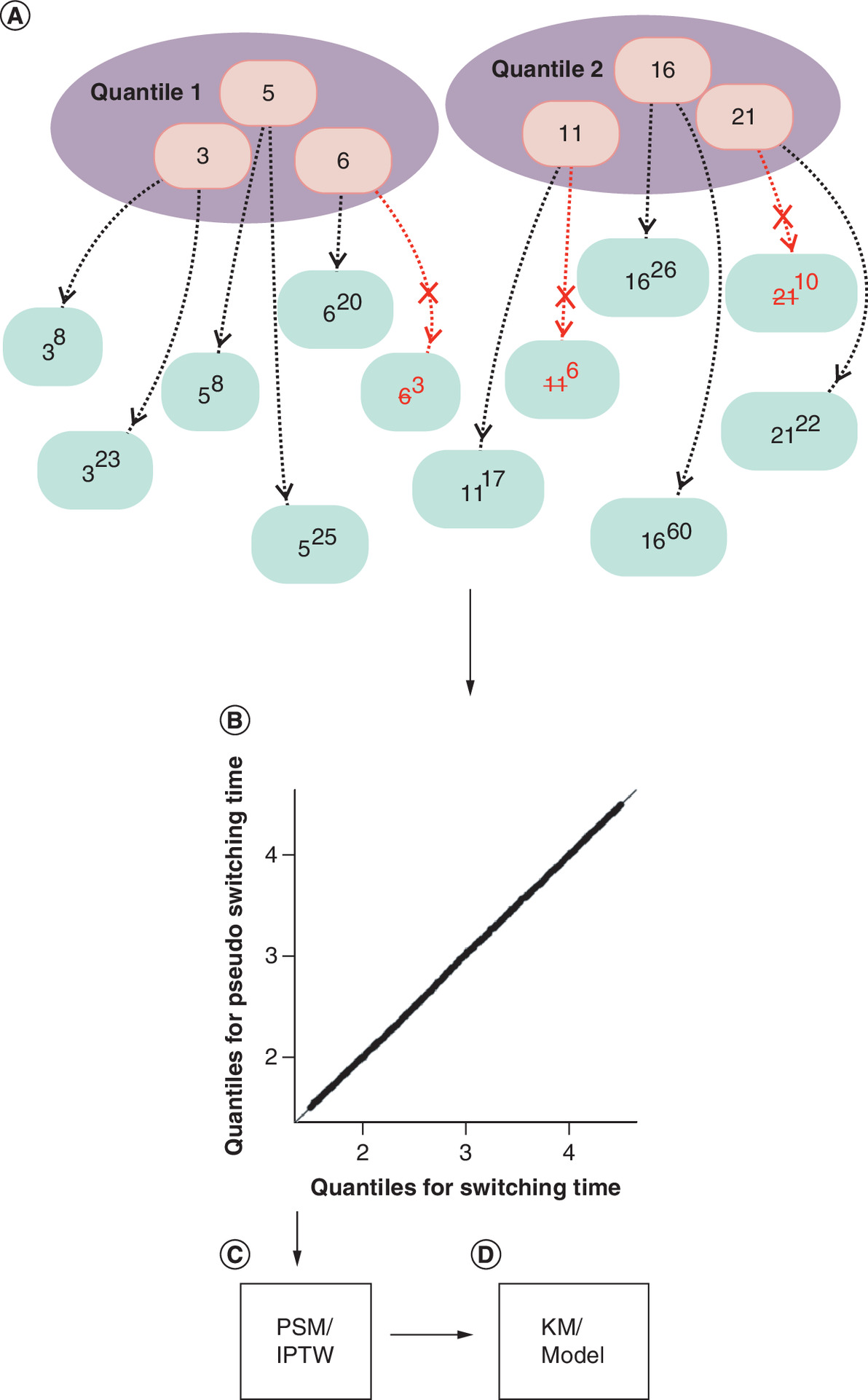
Figure 1. Schematic representation of the developed method.
(A) Assigning switching time from 6 switchers to 12 continuers: switching times (numbers in the orange circles) were divided into two quantiles, drawn from each quantile, and assigned to the continuers (green circles). The base numbers in the green circles were the assigned pseudo-switching times, and the superscripted numbers represent the time from initiation to the end of follow-up. To ensure matched distributions for the assigned pseudo-switching and switching times, the three switching times from each quantile were assigned to six randomly sampled continuers, depicted by dashed lines. Black and red dashed lines indicate assignment success and failure, respectively. In case of assignment failure, a new switching time was re-sampled and re-assigned. Failure occurred when time from initiation to the end of follow-up was shorter than the switching time assigned. (B) Q–Q plot for switching time versus pseudo-switching time: the points lie on a straight line with a slope of 1 and an intercept of 0, indicating similar distribution. (C) Continuers and switchers were propensity score matched or weighted using IPTW if necessary. (D) Results were visualized via a Kaplan–Meier curve, or by fitting a survival model.
IPTW: Inverse probability of treatment weighting; KM: Kaplan–Meier; PSM: Propensity score matching.
Assignment of pseudo-switching times to continuers
Pseudo-switching times were assigned to continuers (as they do not undergo treatment switching) based on the switching times of switchers. To ensure similarity in the distributions of pseudo-switching and switching times, the switchers were divided into K-quantiles based on duration from treatment initiation to treatment switching. Switching times in each quantile are randomly assigned to the continuers. The division of switching times into quantiles and the selection of the switching time from each quantile was to prevent a switching time to be assigned to an excessively large number of continuers and to helps balance the distribution of switching and pseudo-switching times (Figure 1A). While there is an upper limit on the number of continuers being assigned pseudo-switching times from each switcher quantile, there is no strict lower limit, meaning some switching times may be underrepresented among continuers. Therefore, further adjustments may be needed to balance the switching and pseudo-switching times. If an assigned pseudo-switching time exceeds a continuer’s follow-up duration, another switching time is redrawn and re-assign, the assignment is discarded if assignment is unsuccessful after a few rounds. Continuers whose follow-up is shorter than the minimum switching time cannot receive any valid assignment and are excluded.
Match the distributions of pseudo-switching & switching times
Q–Q plots were used to check alignment of distributions of the pseudo-switching and switching times by plotting respective quantiles that correspond to the same probability cutoff (Figure 1B). If the two distributions match, the points corresponding to the same probability cutoff of the distributions should lie on a straight line with a slope of 1 and an intercept of 0.
Matching/weighting of baseline patient characteristics
The continuers and the switchers were further matched/weighted if needed (Figure 1C) based on their baseline characteristics, including risk of events before switching/pseudo-switching. This process would be performed in conjunction with prior steps if the switching/pseudo-switching time requires further matching/weighting. If switching/pseudo-switching time and the baseline characteristics are matched/weighted in separate steps, the balance achieved in previous steps may be impacted.
Compare outcomes
After matching the distributions of pseudo-switching and switching times and balancing patient characteristics, the outcomes of interest were compared (Figure 1D). The outcomes were evaluated from switching/pseudo-switching time to the end of follow-up or occurrence of outcomes or other censoring criteria, whichever occurred first. Kaplan–Meier (KM) curves were generated, and a survival analysis model was used to calculate HRs.
Evaluation of the validity of the developed method through simulation
To evaluate the validity of the proposed method, we simulated cohorts of switchers and continuers who initiated a treatment, with a time-varying confounder measured throughout the follow-up period (Figure 2). The simulation was designed to capture two key challenges that arise when comparing outcomes between switchers and continuers in observational studies: timing bias, which occurs because switchers and continuers are evaluated over different periods of follow-up and confounding by indication, where the decision to switch treatment is influenced by patient characteristics that also affect outcomes.
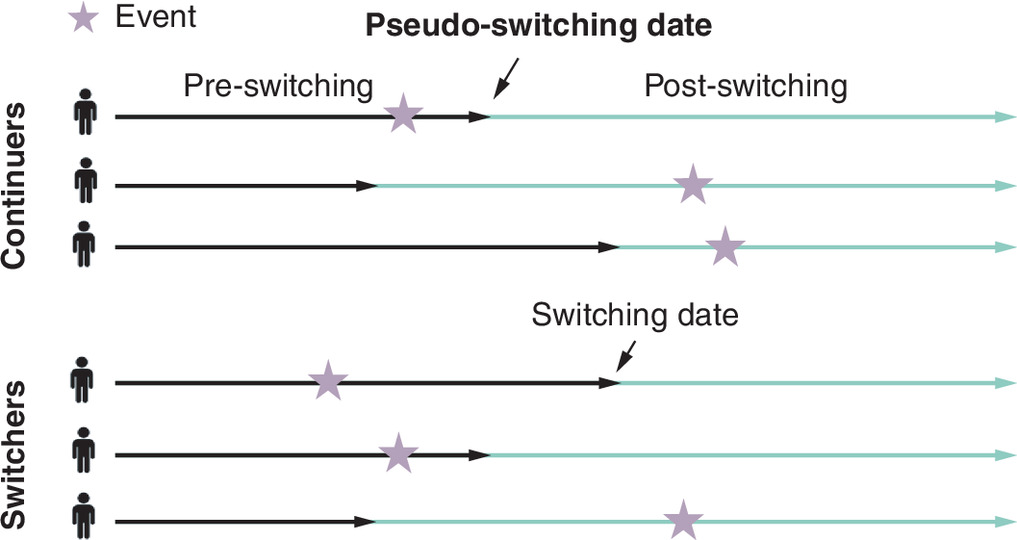
Figure 2. Graph showing the simulation scheme.
Three continuers and three switchers were shown in this case, in which a pseudo-switching date for the continuers and a switching date for the switchers were simulated. The pseudo-switching and switching time are distributed identically. HR between switchers and continuers is different for pre-switch and post-switch, reflecting that pre-switch confound the post-switch.
HR: Hazard ratio.
Follow-up & switching times
For each simulated patient, the total follow-up time from treatment initiation was drawn from a uniform distribution Tj ∼ Uniform (2, 6) years, providing variation in how long patients were observed. Among patients designated as switchers, the switching time was drawn from Sj ∼ Uniform (0.25·Tj, 0.75·Tj) reflecting the fact that switching can occur at various points during treatment but not immediately after initiation or at the very end of follow-up. Each continuer was assigned a hypothetical pseudo-switching time from the same distribution to facilitate evaluation of the method; this pseudo-switching time serves as a reference point for comparing the two groups on equal footing. Note that this hypothetical pseudo-switching time is only used as ground truth; in the analysis, we assign pseudo-switching times using SMARTS.
Time-varying confounder
Rather than using a single baseline measurement, we simulated a continuous confounder measured at regular 0.5-year intervals throughout follow-up, reflecting clinical practice where patient characteristics are monitored over time. The confounder trajectories differed between groups:
•
Continuers: The confounder remained stable around a mean of 2.5 (SD = 0.8), reflecting clinical stability on their current treatment.
•
Switchers: The confounder followed a dynamic trajectory, equaling the continuer value plus a time-varying gap Δ(t) at each time point. This means switchers' confounder values gradually diverge from continuers' values leading up to the switch, then partially converge afterward. The gap evolved linearly in two phases:
(Equation 1a)
(Equation 1b)
where Δ0, ΔS and ΔE denote the gap at baseline, at switching time, and at end of follow-up, respectively. To ensure realistic temporal dependence, where a patient's confounder value at one visit is correlated with values at adjacent visits, the vector of random deviations for patient i was drawn from a multivariate normal distribution:
(Equation 1c)
with an autoregressive covariance structure:
(Equation 1d)
where σ = 0.8 and ρ = 0.9. This structure ensures that confounder values at adjacent time points are highly correlated, with the correlation decaying exponentially over time. The confounder affected the hazard of events with a constant hazard ratio of 2.0 per unit increase (i.e., each one-unit increase in the confounder doubled the hazard of an event).
Clinical scenarios
To demonstrate that SMARTS works under different types of confounding and treatment effects, we simulated two clinical scenarios representing opposite patterns:
•
Sicker switchers, treatment helps (true post-switch HR = 0.7): In this scenario, patients who switch are those experiencing clinical deterioration: they have higher confounder values (e.g., worse lab values or symptom scores) than continuers. The difference in confounder values between switchers and continuers (the ‘gap’) evolves over time: starting at +0.5 at baseline, increasing to a peak of +1.5 at the time of switching (reflecting worsening that triggers the switch), then partially recovering to +0.8 by the end of follow-up. The new treatment is beneficial, reducing the hazard of events by 30%.
•
Healthier switchers, treatment harms (true post-switch HR = 1.5): In this scenario, patients who switch are healthier than continuers: they have lower confounder values and switch for reasons unrelated to disease severity (e.g., cost, convenience and physician preference). The gap trajectory is the mirror image: -0.3 at baseline, reaching -1.5 at switch time, then returning to -0.5 at end of follow-up. The new treatment is harmful, increasing the hazard of events by 50%.
These two scenarios were chosen because they represent clinically plausible but opposing situations. In the first, confounding by indication would make the new treatment appear less effective than it truly is (since switchers are sicker). In the second, confounding would make the new treatment appear more effective than it truly is (since switchers are healthier).
Event generation
Events were generated as a nonhomogeneous Poisson process using a piecewise constant hazard model with 0.5-year segments. The individual hazard for patient i at time t in segment k was:
(Equation 2)
where h0k is the piecewise constant baseline hazard for segment k, is the confounder value measured at the last assessment before the switch time, βc = log (2.0) is the confounder effect (HR = 2.0 per unit), βT = log (HRtrue) is the treatment effect and Zi (t) is the treatment indicator (1 for switchers after switching, 0 otherwise). An important design choice was that event generation used the confounder value measured at (pseudo-) switching time for both the pre-switch and post-switch periods. This ensures consistency with the analysis methods, which adjust for the confounder at (pseudo-)switching time. Because this confounder value is measured before the switch occurs, it is not a mediator of the treatment effect: it reflects the patient’s clinical state leading up to the switch decision, not a consequence of the new treatment. Using post-switch confounder values would risk adjusting away part of the treatment effect, since post-switch changes in the confounder may be caused by the new treatment itself.
Hazard trends
The direction and magnitude of timing bias depend on how the baseline hazard changes over time. To examine this, we evaluated three hazard trend scenarios:
•
Constant hazard: h0k = λ0 where λ0 = 0.02. This serves as a control condition where no timing bias is expected, since the hazard is the same regardless of when a patient is evaluated.
•
Increasing hazard: h0k = λ0 (1 + α · tk) with α = 0.25. This represents diseases that worsen over time, and creates upward timing bias: the conventional approach overestimates the HR because continuers are evaluated during an earlier, lower-hazard period.
•
Decreasing hazard: h0k = λ0 max(0.1, 1 – α · tk) with α = 0.25. This represents improving prognosis over time (e.g., decreasing risk after an acute event), and creates downward timing bias: the conventional approach underestimates the HR.
Factorial design
Simulations were conducted under a 2 × 3 factorial design crossing clinical scenario (sicker switchers vs healthier switchers) with hazard trend (constant vs increasing vs decreasing), yielding six conditions. For each condition, 100 datasets of 4000 patients (2000 switcher – continuer pairs) were simulated. All simulations were performed using R statistical programming software.
Analysis of the simulated data
Each simulated dataset was analyzed using five methods, applied under both the conventional approach (continuers were evaluated from treatment initiation to the end of follow-up) and the SMARTS approach (continuers were evaluated from treatment pseudo-switching to the end of follow-up), for a total of ten analyses per dataset:
•
Naive: Unadjusted Cox proportional hazards regression comparing switchers and continuers, without adjusting for confounders.
•
Adjusted (Adj): Cox regression including the confounder value at (pseudo-)switching time as a covariate.
•
Propensity score matching (PSM): Switchers and continuers were matched on the estimated propensity score (probability of switching) based on the confounder at (pseudo-)switching time.
•
Inverse probability of treatment weighting (IPTW): Patients were weighted by the inverse of their estimated probability of being in their observed group, targeting the average treatment effect (ATE) in the combined population.
•
Standardized morbidity ratio weighting (SMR): Continuers were weighted to match the covariate distribution of switchers, targeting the average treatment effect in the treated (ATT) – i.e., the effect specifically among those who switched.
Under the conventional approach, continuers were evaluated from treatment initiation to the end of follow-up, using their baseline confounder value at treatment initiation. Switchers were evaluated from switching time to the end of follow-up, using their confounder at switch time. This creates two sources of potential bias: the follow-up periods are not aligned in time since treatment initiation, and the confounder values are measured at different time points (baseline for continuers vs switch time for switchers).
Under the SMARTS approach, continuers were assigned pseudo-switching times using the SMARTS algorithm, and both groups were evaluated from their (pseudo-)switching time to the end of follow-up. Confounder values at (pseudo-)switching time were used for adjustment in both groups, ensuring that follow-up periods and confounder measurements are aligned.
Given that the assignment of pseudo-switching times to continuers is random, results may vary across different assignments. To account for this variability, 1000 independent random pseudo-switching time assignments were performed per dataset, and the resulting hazard ratio estimates were averaged to produce a single, more stable estimate per dataset.
Application of the proposed method to a real-world study
Nonvalvular atrial fibrillation (NVAF) is associated with an increased risk of developing stroke. Direct oral anticoagulants such as apixaban and rivaroxaban are considered the standard of care for stroke prevention in patients with NVAF in the USA [7–10], and direct oral anticoagulants switching occurs frequently in clinical practice [32] as a result of clinical events such as stroke/bleeding, other side effects of the medication [33–35], or formulary restrictions [36]. Application of the method to compare clinical outcomes between patients with NVAF who initiated rivaroxaban and then switched to apixaban versus patients continuing on rivaroxaban is described elsewhere [31]. To demonstrate how the study results can be impacted by the application of our method, we re-analyze the data comparing the risk of major bleeding (MB) and stroke events for the rivaroxaban initiators using the following three methods, prompted by the fact that patients who switched from rivaroxaban to apixaban have worse baseline characteristics compared with patients who continued rivaroxaban, aligning with what was described in the simulation. We did not re-analyze the apixaban initiators because patients who switched from apixaban to rivaroxaban have similar baseline characteristics with patients who continued apixaban.
•
No pseudo-switch: There was no pseudo-switching time assigned to continuers. Continuers were evaluated from treatment initiation to the end of follow-up for the occurrence of the MB and stroke event. The switchers were evaluated from the switching time to the end of follow-up for the occurrence of the events.
•
Assign pseudo-switch: Continuers were assigned pseudo-switching time. Both continuers and switchers were evaluated from treatment initiation to pseudo-switching/switching time and from pseudo-switching/switching to end of follow-up. Matching of patient characteristics was not performed.
•
Assign pseudo-switch + propensity score match (PSM): Similar to scenario 2, continuers were assigned pseudo-switching time. PSM was performed to ensure the risk of event occurrence before switching/pseudo-switching was balanced between the two cohorts.
Using Q–Q plots, we present how the distribution of pseudo-switching times for continuers compared with the distribution of switching times for switchers after utilizing the proposed method. Using forest plot, we compare the incidence rate and HRs obtained using the three methods described above.
Results
Validity of the proposed method
KM illustration
To illustrate the impact of timing bias and the correction provided by SMARTS, we present KM curves for both clinical scenarios under increasing hazard (Figures 3 & 4).
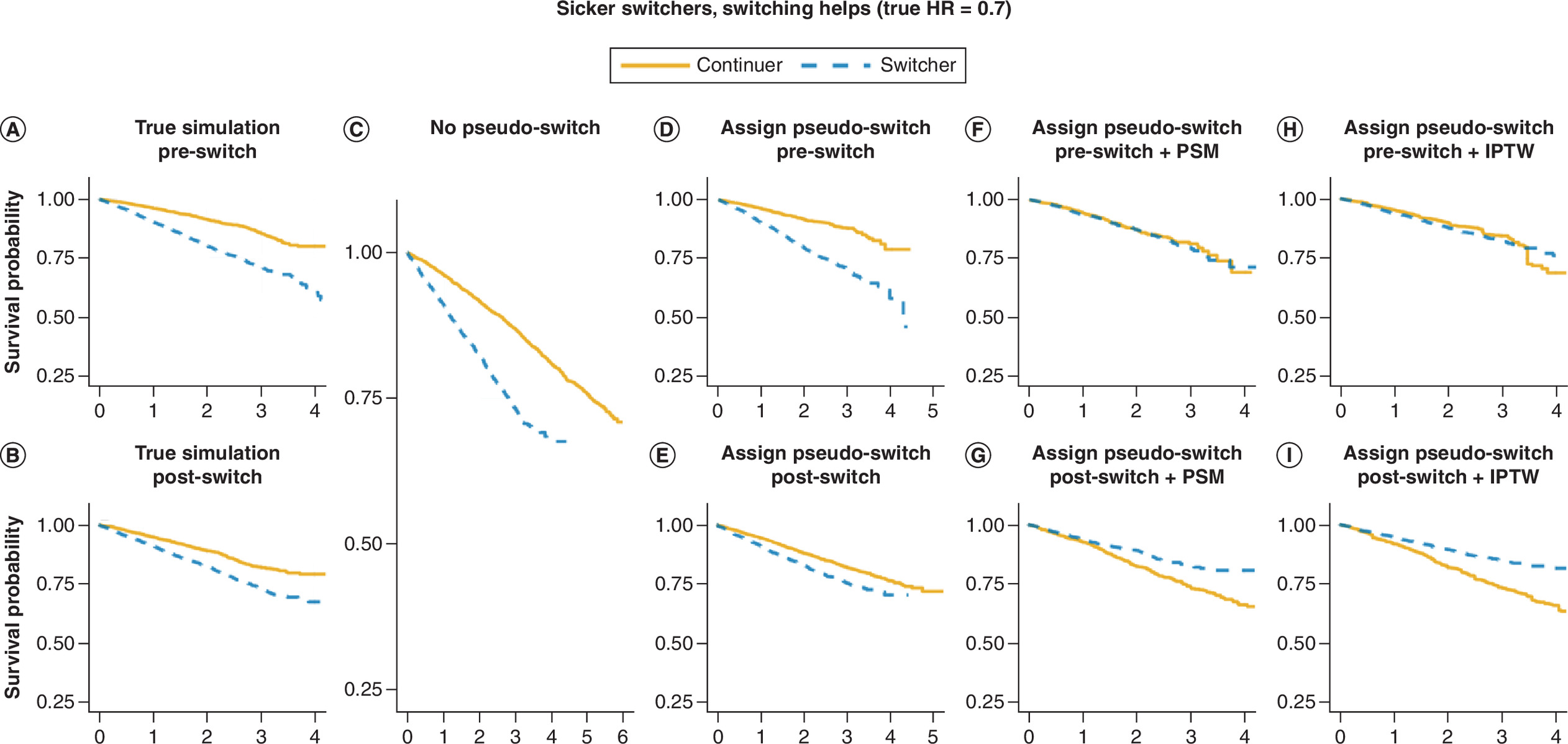
Figure 3. Kaplan–Meier curves for scenarios where switchers are sicker prior to switching and become healthier after switching due to the new treatment’s effect.
Continuers plotted in yellow, switchers plotted in blue. KM plots are, respectively, for (A) event outcome for pre-switch for the true simulation; (B) event outcome for post-switch for the true simulation; (C) event outcome in the follow-up period from treatment initiation to follow-up end for the continuers, and from treatment switching to follow-up end for the switchers; (D) event outcome for pre-switch period after assigning pseudo-switching time; (E) event outcome for post-switch period after assigning pseudo-switching time; (F) event outcome similar to scenario in D, but further matched continuers and switchers based on the pseudo-switching time/switching time and event risk pre-switch; (G) event outcome similar with scenario in E, but further matched continuers and switchers based on the pseudo-switching time/switching time and risk of pre-switch. (H) Event outcome similar to scenario in D, but further weighted continuers and switchers on event risk pre-switch using IPTW; (I) event outcome similar with scenario in E, but further weighted continuers and switchers based on the pseudo-switching time/switching time and risk of event pre-switch using IPTW.
HR: Hazard ratio; IPTW: Inverse probability of treatment weighting; KM: Kaplan–Meier; PSM: Propensity score matching.
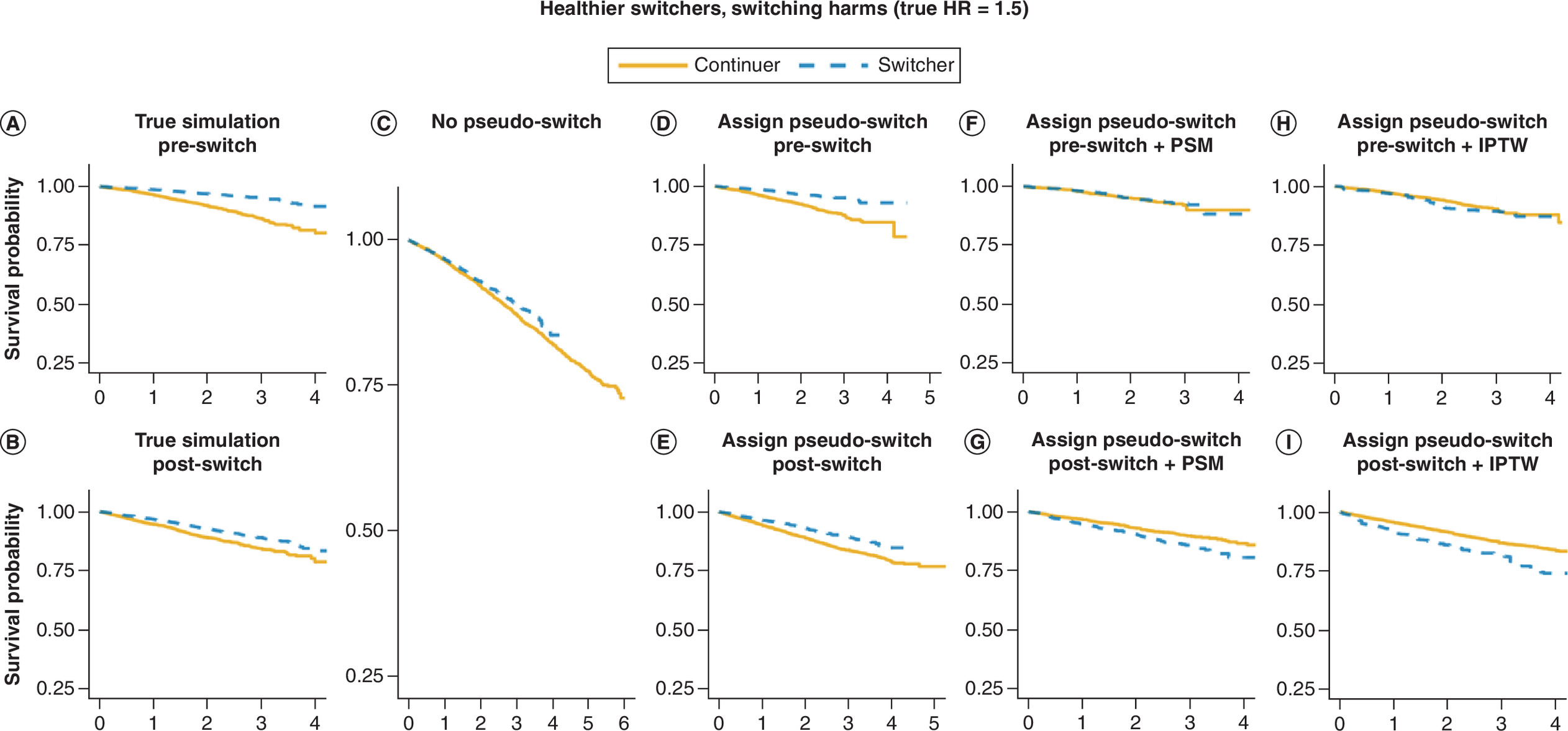
Figure 4. Kaplan–Meier curves for scenarios where switchers are healthier prior to switching and become sicker after switching because the new treatment does not help.
Continuers plotted in yellow, switchers plotted in blue. KM plots are, respectively, for (A) event outcome for pre-switch for the true simulation; (B) event outcome for post-switch for the true simulation; (C) event outcome in the follow-up period from treatment initiation to follow-up end for the continuers, and from treatment switching to follow-up end for the switchers; (D) event outcome for pre-switch period after assigning pseudo-switching time; (E) event outcome for post-switch period after assigning pseudo-switching time; (F) event outcome similar to scenario in D, but further matched continuers and switchers based on the pseudo-switching time/switching time and event risk pre-switch; (G) event outcome similar with scenario in E, but further matched continuers and switchers based on the pseudo-switching time/switching time and risk of pre-switch. (H) Event outcome similar to scenario in D, but further weighted continuers and switchers on event risk pre-switch using IPTW; (I) event outcome similar with scenario in E, but further weighted continuers and switchers based on the pseudo-switching time/switching time and risk of event pre-switch using IPTW.
HR: Hazard ratio; IPTW: Inverse probability of treatment weighting; KM: Kaplan–Meier; PSM: Propensity score matching.
For the ‘sicker switchers, treatment helps’ scenario (true HR = 0.7; Figure 3), the KM curves from the true simulated data show that switchers had a higher risk of events than continuers before switching (Figure 3A), consistent with the higher confounder values assigned to switchers. After switching, the KM curves (Figure 3B) show that switchers had a higher event rate than continuers, reflecting the beneficial treatment effect was confounded by the confounders.
When continuers were not assigned pseudo-switching times and were evaluated from treatment initiation (the conventional approach; Figure 3C), the pattern was similar. However, including the pre-switch period introduces a different time period with a different baseline hazard than the post-switch period, which could result in more biased estimates, as shown in the factorial simulation results (Figure 5).
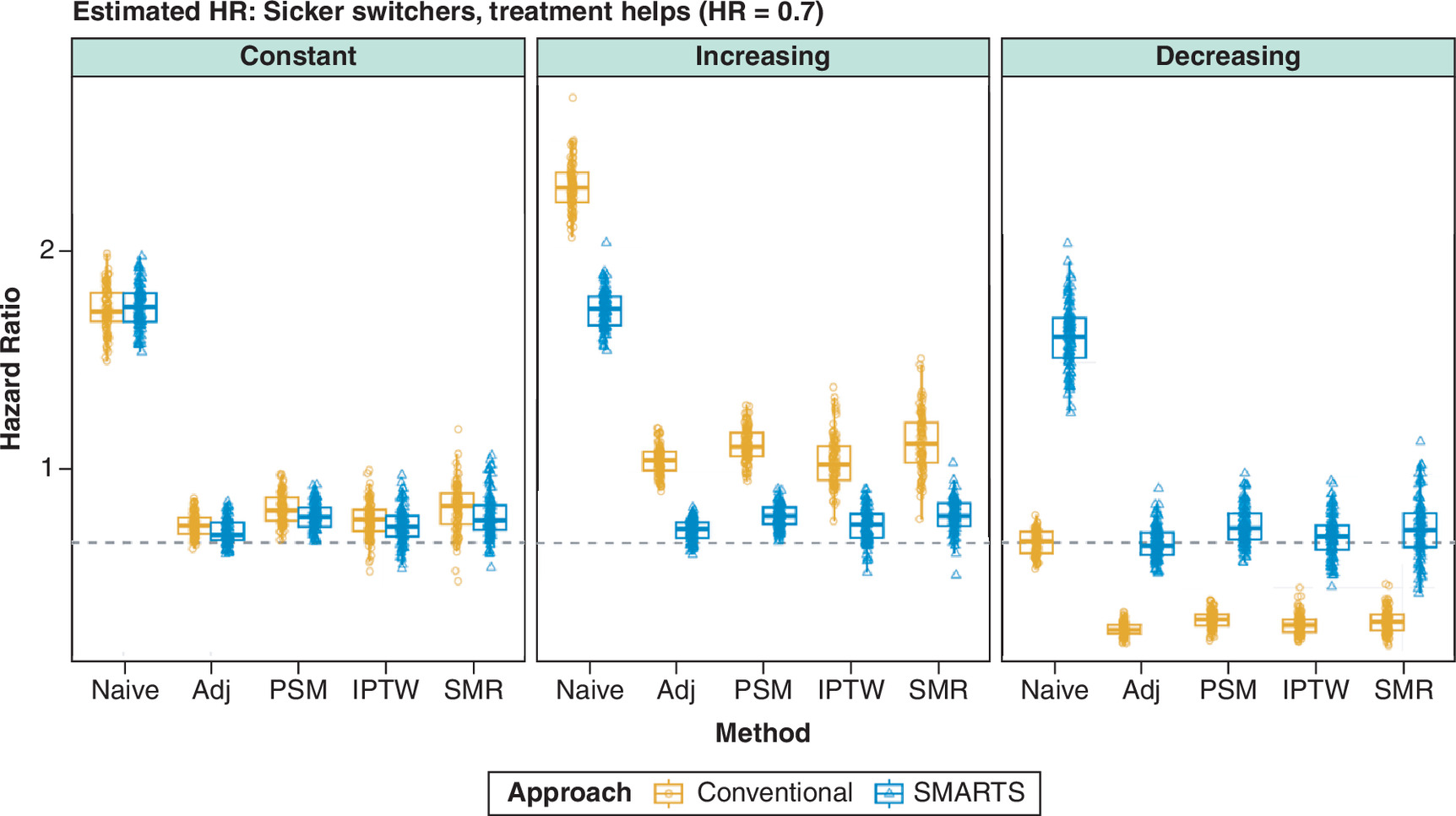
Figure 5. Distribution of estimated hazard ratios across 100 simulated datasets under the sicker switchers, treatment helps scenario (true HR = 0.7, dashed line).
Columns represent three baseline hazard trends (constant, increasing and decreasing). Five analysis methods are compared: naive (unadjusted), adjusted (Adj), PSM, IPTW and SMR. Orange boxes indicate the conventional approach (continuers evaluated from treatment initiation); blue boxes indicate the SMARTS approach (continuers assigned pseudo-switching times). Each point represents one simulated dataset. Under increasing and decreasing hazard, the conventional approach produces substantially biased estimates, while SMARTS combined with confounder adjustment recovers estimates close to the true HR.
Adj: Adjusted; HR: Hazard ratio; IPTW: Inverse probability of treatment weighting; PSM: Propensity score matching; SMR: Standardized morbidity ratio weighting.
After assigning pseudo-switching times using SMARTS (Figure 3D & E), the pre-switch and post-switch KM curves exhibited a pattern similar to that of the unadjusted data, as confounding between switchers and continuers remained unaddressed by time alignment alone. The benefit of pseudo-switching time assignment became apparent only after additional confounder adjustment. PSM (Figure 3F & G) and inverse probability of treatment weighting (Figure 3H & I) balanced the confounder distribution at the time of switching, and the resulting post-switch survival curves more closely approximated the true treatment effect.
For the ‘healthier switchers, treatment harms’ scenario (true HR = 1.5), an analogous set of KM curves showed the mirror-image pattern. In the true data, switchers had lower pre-switch event risk (due to lower confounder values) and higher post-switch event risk (due to the harmful treatment effect). The conventional approach again distorted the comparison, while SMARTS with confounder adjustment recovered the true treatment effect pattern.
Results for factorial simulation
| Hazard | Approach | Naive | Adj | PSM | IPTW | SMR | |
|---|---|---|---|---|---|---|---|
| Sicker switchers, treatment helps (true HR = 0.70) | Constant | Conventional | 1.74 (0.10) | 0.78 (0.05) | 0.85 (0.07) | 0.80 (0.08) | 0.85 (0.11) |
| SMARTS | 1.75 (0.10) | 0.75 (0.05) | 0.82 (0.06) | 0.77 (0.08) | 0.82 (0.10) | ||
| Increasing | Conventional | 2.29 (0.11) | 1.06 (0.06) | 1.14 (0.07) | 1.06 (0.11) | 1.15 (0.13) | |
| SMARTS | 1.74 (0.09) | 0.76 (0.05) | 0.82 (0.05) | 0.78 (0.07) | 0.82 (0.07) | ||
| Decreasing | Conventional | 0.70 (0.05) | 0.31 (0.03) | 0.36 (0.04) | 0.34 (0.05) | 0.35 (0.05) | |
| SMARTS | 1.61 (0.14) | 0.70 (0.07) | 0.78 (0.09) | 0.73 (0.10) | 0.76 (0.13) | ||
| Healthier switchers, treatment harms (true HR = 1.50) | Constant | Conventional | 0.62 (0.04) | 1.35 (0.13) | 1.30 (0.15) | 1.42 (0.23) | 1.33 (0.21) |
| SMARTS | 0.62 (0.04) | 1.44 (0.15) | 1.38 (0.15) | 1.46 (0.23) | 1.42 (0.22) | ||
| Increasing | Conventional | 0.84 (0.05) | 1.82 (0.13) | 1.70 (0.15) | 1.80 (0.19) | 1.72 (0.26) | |
| SMARTS | 0.63 (0.04) | 1.43 (0.10) | 1.36 (0.10) | 1.41 (0.14) | 1.37 (0.18) | ||
| Decreasing | Conventional | 0.26 (0.03) | 0.56 (0.08) | 0.55 (0.09) | 0.61 (0.18) | 0.54 (0.11) | |
| SMARTS | 0.60 (0.07) | 1.41 (0.22) | 1.38 (0.24) | 1.46 (0.46) | 1.40 (0.36) |
Two clinical scenarios were evaluated: sicker switchers where treatment helps (true HR = 0.70) and healthier switchers where treatment harms (true HR = 1.50). Three hazard trends were examined: constant, increasing, and decreasing. The conventional approach evaluates continuers from treatment initiation; the SMARTS approach assigns pseudo-switching times to continuers from the empirical switcher distribution. Five Cox regression methods were applied: naive (unadjusted), covariate-adjusted (Adj), PSM, IPTW and SMR. For each dataset under the SMARTS approach, results were averaged over 1000 independent random pseudo-switching time assignments. Values closer to the true HR with smaller SD indicate better performance.
Adj: Adjusted; HR: Hazard ratio; IPTW: Inverse probability of treatment weighting; PSM: Propensity score matching; SMR: Standardized morbidity ratio weighting.
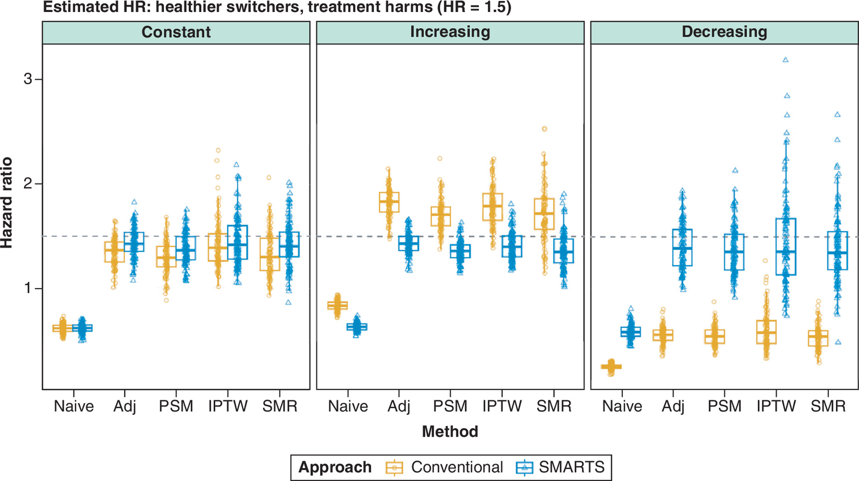
Figure 6. Distribution of estimated hazard ratios across 100 simulated datasets under the healthier switchers, treatment harms scenario (true HR = 1.5, dashed line).
Columns represent three baseline hazard trends (constant, increasing and decreasing). Five analysis methods are compared: naive (unadjusted), adjusted (Adj), PSM, IPTW and SMR. Orange boxes indicate the conventional approach (continuers evaluated from treatment initiation); blue boxes indicate the SMARTS approach (continuers assigned pseudo-switching times). Each point represents one simulated dataset. Under increasing and decreasing hazard, the conventional approach produces substantially biased estimates, while SMARTS combined with confounder adjustment recovers estimates close to the true HR.
Adj: Adjusted; HR: Hazard ratio; IPTW: Inverse probability of treatment weighting; PSM: Propensity score matching; SMR: Standardized morbidity ratio weighting.
Results for simulation with constant hazard
When the baseline hazard was constant over time (Figures 5 & 6, left panel), the timing mismatch between evaluating continuers from treatment initiation and switchers from their switch date did not introduce systematic bias, because the baseline event rate was the same at both time points. After confounder adjustment, both the conventional and SMARTS approaches yielded estimates close to the true hazard ratio. For example, in the sicker-switchers scenario (true HR = 0.70) (Figure 5), the adjusted conventional estimate was 0.78 (SD 0.05) and the SMARTS estimate was 0.75 (SD 0.05); results were comparable across all adjustment methods (Table 1). SMARTS produced marginally closer estimates, likely because measuring confounders at the pseudo-switching time, rather than at treatment initiation, provides better alignment with the confounder values of switchers at the time of their switch.
Results for simulation with changing hazard
Comparing outcomes between switchers and continuers is subject to two sources of bias. First, switchers have different pre-switch risk profiles than continuers: sicker in Scenario 1, healthier in Scenario 2, which confounds the post-switch hazard ratio if not properly adjusted. Second, the conventional approach evaluates continuers from treatment initiation but switchers from their switching time; when the baseline hazard changes over time, the two groups are compared under different risk conditions, introducing timing bias. These two biases compound each other: the conventional approach not only fails to account for the different risk profiles, but also measures confounders at treatment initiation for continuers, which do not reflect the clinical state they would have at the later switching time. Even after confounder adjustment, the conventional approach produced substantially biased estimates when hazard varied over time (Figures 5 & 6, middle and right panels).
Under increasing hazard (Figure 5, middle panel), the early period (when continuers are evaluated) has low baseline hazard, while the later period (when switchers are evaluated) has high baseline hazard. If early period of continuers are included in the analysis (conventional approach), it makes continuers appear healthier than they would be at the time of switching, exaggerating the contrast with switchers and inflating the estimated hazard ratio. In the sicker-switchers scenario (true post-switching HR = 0.70), the adjusted conventional estimate was 1.06 (SD 0.06), reversing the apparent direction of the treatment effect and suggesting harm when the true effect was protective. SMARTS corrected this to 0.76 (SD 0.05) by aligning both groups at comparable time points, ensuring that confounders are measured at the same stage of disease progression. A similar pattern of upward bias was observed in the healthier-switchers scenario (Figure 6, middle panel; Table 1).
Under decreasing hazard, the reverse occurs: the early period has high baseline hazard, If early period of continuers are included in the analysis (conventional approach), it makes continuers appear sicker than they would be at the later switching time. This deflates the estimated hazard ratio by inflating the event rate among continuers relative to switchers who are evaluated during the later, lower-hazard period. In the healthier-switchers scenario (true post-switching HR = 1.50), the adjusted conventional estimate was 0.56 (SD 0.08), suggesting benefit when the true effect was harmful (Figure 6, right panel). SMARTS corrected this to 1.41 (SD 0.22). Complete results across all scenarios and methods are shown in Table 1 & Figures 5 & 6.
Opposing biases can mask the problem
An instructive pattern emerged in the sicker-switchers scenario under decreasing hazard. The naive (unadjusted) conventional analysis recovered the true hazard ratio almost exactly (mean HR = 0.70, SD 0.05), despite making no correction for either confounding or timing. This apparent accuracy arose because two opposing biases happened to cancel: confounding bias from the sicker switcher population (which inflates the hazard ratio) and timing bias from including continuers’ early high-hazard period (which deflates it). When confounding was appropriately adjusted for and removed one of the two biases, the timing bias was unmasked, and the adjusted conventional estimate dropped to 0.31 (SD 0.03), massively overestimating the treatment benefit.
This finding illustrates a practical danger: a naive conventional analysis may yield a plausible-looking result, providing false reassurance that the analysis is sound. The underlying biases become apparent only when one is partially corrected, making the estimate paradoxically worse. SMARTS addresses both sources of bias simultaneously: temporal alignment removes the timing component, and confounder adjustment at the pseudo-switching time addresses the confounding component, yielding an estimate of 0.70 (SD 0.07).
Choice of confounder adjustment method
Regression adjustment, PSM, IPTW and SMR weighting all produced comparable point estimates when combined with SMARTS (Table 1). However, IPTW and SMR exhibited higher variability. For example, in the healthier-switchers scenario under decreasing hazard, SMARTS with regression adjustment yielded a mean HR of 1.41 (SD 0.22), whereas SMARTS with IPTW yielded 1.46 (SD 0.46). This higher variability is a well-known property of inverse probability weighting when propensity scores approach 0 or 1, and was observed under both the conventional and SMARTS approaches at comparable magnitudes, confirming that it reflects the weighting method rather than the pseudo-switching time assignment. Regression adjustment and PSM provided the most stable estimates across all scenarios.
Application to a real-world study
As described elsewhere [31], NVAF patients initiating rivaroxaban between 1 January 2013 and 31 December 2021 were identified Using Optum’s de-identified Clinformatics®Data Mart Database. Pseudo-switching times were assigned to rivaroxaban continuers using the method described in this article. Switchers and continuers were matched at a ratio of 1:5, resulting in 2873 rivaroxaban-to-apixaban switchers to be matched with 14,365 rivaroxaban continuers. Figure 7 indicates matching distributions of pseudo-switching and switching times.
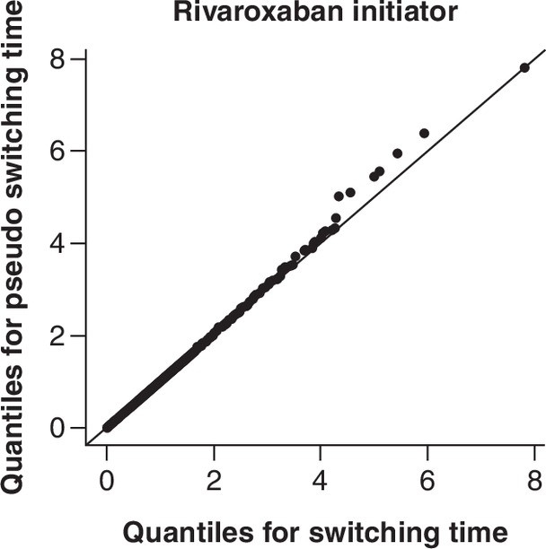
Figure 8 presented the IRs and HRs for risk of MB and stroke between switchers and continuers for the rivaroxaban initiators, re-analyzed from the study described in Deitelzweig et al. [31]. When continuers were not assigned pseudo-switching time and were evaluated from treatment initiation to the end of follow-up and switchers were evaluated from switching to end of follow-up, the HR of MB and stroke between switchers and continuers for rivaroxaban initiators were 0.77 and 1.02. After assigning pseudo-switching times to the continuers and evaluating from switching/pseudo-switching to follow-up end, the HR of MB and stroke were 0.69 and 0.94. Following further balancing the continuers and the switchers, the HR of MB and stroke were 0.49 and 0.74.
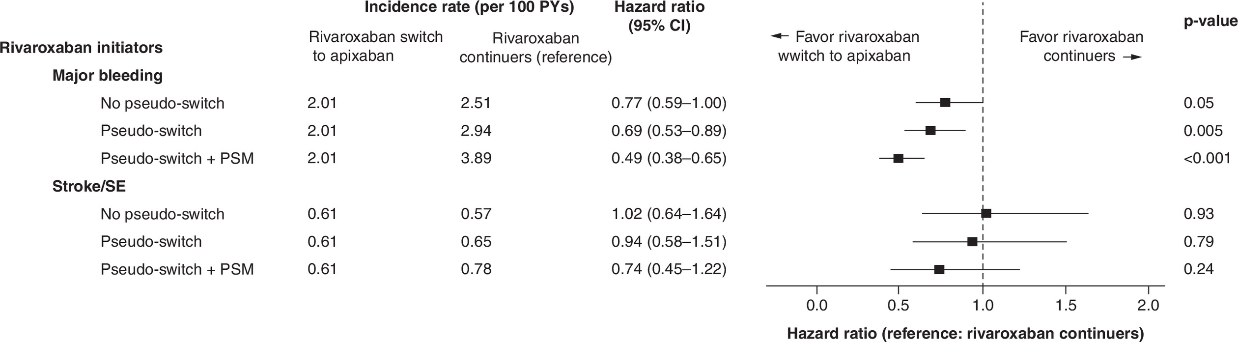
Figure 8. Forest plot showing incidence rates and hazard ratios for nonvalvular atrial fibrillation patients initiating rivaroxaban, re-analyzed using different methods.
CI: Confidence interval; HR: Hazard ratio; IR: Incidence rate; PSM: Propensity score matching; PY: Person year; SE: Systemic embolism.
Discussion
We developed and validated SMARTS, a method for comparing outcomes between treatment switchers and continuers in routine clinical practice. The method assigns pseudo-switching times to continuers from the empirical distribution of actual switching times, aligning the time origins from which outcomes are evaluated. Our factorial simulation demonstrated that this temporal alignment substantially reduces bias when the baseline hazard changes over time: under increasing or decreasing hazard, the conventional approach produced severely biased estimates (e.g., adjusted HR = 1.06 vs true HR = 0.70 under increasing hazard in the sicker-switchers scenario), while SMARTS combined with confounder adjustment recovered estimates close to the true value across all scenarios. Under constant hazard, both approaches performed well, confirming that timing bias is the specific issue SMARTS addresses.
Several existing methods address treatment switching, and it is important to clarify how SMARTS relates to these. The two-stage methods in NICE TSD 16 [23–25] address patients who switch from a control to the active treatment in randomized trials, aiming to estimate the counterfactual outcome had no switching occurred. SMARTS addresses a fundamentally different question: directly comparing outcomes between patients who switch away from an initial treatment versus those who continue, without constructing counterfactual outcomes. Marginal structural models and g-estimation [13,15,37–39] address time-varying confounding along the treatment trajectory but do not resolve the index date problem – without a valid starting point for evaluating continuers, any downstream analysis carries timing bias when hazard changes over time. SMARTS is complementary to these approaches: it provides the temporal alignment, after which any confounding adjustment method can be applied. The prevalent new-user design of Suissa et al. [12] also addresses the index date problem but matches on calendar date rather than time since treatment initiation. We argue that treatment duration is the more clinically appropriate matching axis, as patients at the same calendar date may be at very different stages of their treatment trajectory. Calendar-time matching may be preferred when secular trends are the dominant concern.
The proposed method has several strengths: it addresses a practical problem often overlooked in observational studies, is agnostic to the downstream confounding adjustment strategy, does not require knowledge of the reason for switching, and is straightforward to implement via the publicly available SMARTS R package. Several limitations should be acknowledged. The random assignment of pseudo-switching times introduces variability, which we mitigated by averaging over 1000 independent assignments per dataset. Continuers with follow-up shorter than the minimum switching time are excluded; the exclusion rate should be reported. The method assumes noninformative censoring conditional on measured confounders; combining SMARTS with inverse probability of censoring weighting could address informative censoring in future work. Finally, the analysis adjusts for confounders measured at (pseudo-)switching time but not for post-switch changes [40], which may be mediators of the treatment effect rather than confounders.
In conclusion, SMARTS provides a practical tool for researchers evaluating treatment switching in routine clinical practice. By aligning the time origins for switchers and continuers, the method eliminates timing bias that can reverse the apparent direction of the treatment effect. Combined with confounder adjustment at the (pseudo-)switching time, it substantially reduced bias across a range of simulated scenarios and was successfully applied to a real-world study of anticoagulant switching in patients with non-valvular atrial fibrillation.
Conclusion
We have developed a method to address the methodological issues associated with outcomes comparisons between switchers and continuers in routine clinical practice. The simulation demonstrated that the method is valid and reduced the magnitude of bias in comparing outcomes between switchers and continuers. This method has been successfully applied to a recently published real-world study. Additional application will further confirm the utility of this method.
Summary points
•
When researchers need to assess the impact of treatment switch, a common challenge is to identify the appropriate index date for measuring clinical outcomes in continuers for comparison with switchers (for whom the switching date could serve as the index date). The two cohorts (continuers and switchers) usually have very different risk profiles and the risk of a clinical event of interest usually changes over time.
•
We have developed a method to address the methodological challenges by assigning pseudo-switching times to the continuers with matched distribution to the switching times for switchers.
•
The method further matched/weighted both groups to ensure comparable comorbidities and risk of clinical events before switching/pseudo-switching.
•
The method was validated by simulating a cohort of switchers and continuers with a specific hazard ratio (HR) of a simulated clinical event between the two groups.
•
The validation showed that our method of assigning pseudo-switching times to the continuers and matching/weighting the distribution of the switching times/pseudo-switching times and the preswitching risk of event, yielded HR estimates closer to the true simulated HR.
•
Application of the method to a real-world study improved the distribution of pre-switch times between rivaroxaban continuers and rivaroxaban-to-apixaban switchers.
Author contributions
All authors substantially contributed to the development and critical revision of the intellectual content and approved the final version.
Financial disclosure
Bristol Myers Squibb (US) and Pfizer (US) Alliance provided funding for this research.
Competing interests disclosure
A Kang and X Li are employees and shareholders of Bristol Myers Squibb, a study sponsor. C Gao, J Jiang and N Atreja were employees and shareholders of Bristol Myers Squibb at time of study. X Luo is an employee and shareholder of Pfizer, a study sponsor. The authors have no other competing interests or relevant affiliations with any organization or entity with the subject matter or materials discussed in the manuscript apart from those disclosed.
Writing disclosure
No funded writing assistance was utilized in the production of this manuscript.
Software availability
An implementation of the SMARTS method is available as an R package at https://github.com/chuangao/SMARTS
Open access
This work is licensed under the Attribution-NonCommercial-NoDerivatives 4.0 Unported License. To view a copy of this license, visit https://creativecommons.org/licenses/by-nc-nd/4.0/
References
Papers of special note have been highlighted as: • of interest
1.
Latimer NR. Treatment switching in oncology trials and the acceptability of adjustment methods. Expert Rev. Pharmacoecon. Outcomes Res. 15(4), 561–564 (2015).
2.
Baker CL, Dhamane AD, Rajpura J et al. Switching to another oral anticoagulant and drug discontinuation among elderly patients with nonvalvular atrial fibrillation treated with different direct oral anticoagulants. Clin. Appl. Thromb. Hemost. 25, 1076029619870249 (2019).
3.
Sullivan TR, Latimer NR, Gray J, Sorich MJ, Salter AB, Karnon J. Adjusting for treatment switching in oncology trials: a systematic review and recommendations for reporting. Value Health 23(3), 388–396 (2020).
4.
Guinart D, Varma K, Segal Y, Talasazana N, Correll CU, Kane JM. Reasons for antipsychotic treatment switch: a systematic retrospective review of prescription records and prescriber notes. J. Clin. Psychiatry 83(5), 42616 (2022).
5.
Singh H, Wilson L, Tencer T, Kumar J. Systematic literature review of real-world evidence on dose escalation and treatment switching in ulcerative colitis. ClinicoEcon. Outcomes Res. 15, 125–138 (2023).
6.
Baker CL, Dhamane AD, Mardekian J et al. Comparison of drug switching and discontinuation rates in patients with nonvalvular atrial fibrillation treated with direct oral anticoagulants in the United States. Adv. Ther. 36(1), 162–174 (2019).
7.
Chen A, Stecker E, Warden BA. Direct oral anticoagulant use: a practical guide to common clinical challenges. J. Am. Heart Association. 9(13), e017559 (2020).
8.
Zhu J, Alexander GC, Nazarian S, Segal JB, Wu AW. Trends and variation in oral anticoagulant choice in patients with atrial fibrillation, 2010–2017. Pharmacotherapy 38(9), 907–920 (2018).
9.
Ezekowitz MD, Pollack CV Jr, Halperin JL et al. Apixaban compared to heparin/vitamin k antagonist in patients with atrial fibrillation scheduled for cardioversion: The EMANATE trial. Eur. Heart J. 39(32), 2959–2971 (2018).
10.
Patel MR, Mahaffey KW, Garg J et al. Rivaroxaban versus warfarin in nonvalvular atrial fibrillation. N. Engl. J. Med. 365(10), 883–891 (2011).
11.
Liu F, Panagiotakos D. Real-world data: a brief review of the methods, applications, challenges and opportunities. BMC Med. Res. Methodol. 22(1), 287 (2022).
12.
Suissa S, Moodie EE, Dell'Aniello S. Prevalent new-user cohort designs for comparative drug effect studies by time-conditional propensity scores. Pharmacoepidemiol. Drug Saf. 26(4), 459–468 (2017).
13.
Robins JM, Tsiatis AA. Correcting for non-compliance in randomized trials using rank preserving structural failure time models. Commun. Stat. Theory Methods 20(8), 2609–2631 (1991).
• Laid out the theoretical foundation of the counterfactual rank preserving structural failure time model for randomized controlled trial.
14.
White IR, Walker S, Babiker AG, Darbyshire JH. Impact of treatment changes on the interpretation of the Concorde trial. AIDS 11(8), 999–1006 (1997).
15.
White IR, Babiker AG, Walker S, Darbyshire JH. Randomization-based methods for correcting for treatment changes: examples from the Concorde trial. Stat. Med. 18(19), 2617–2634 (1999).
• Illustrates the basic principle of Rank Preserving Structural Failure Time Models using the Concorde trial as an example.
16.
Allison A, White IR, Bond S. rpsftm: an R package for rank preserving structural failure time models. R. J. 9(2), 342–353 (2017).
• Introduces and implemented the Rank Preserving Structural Failure Time Models in the statistical language of R.
17.
Frangakis CE, Rubin DB. Principal stratification in causal inference. Biometrics 58(1), 21–29 (2002).
18.
Barnard J, Frangakis CE, Hill JL, Rubin DB. Principal stratification approach to broken randomized experiments. J. Am. Stat. Assoc. 98(462), 299–323 (2003).
19.
Mattei A, Mealli F, Din P. Assessing causal effects in the presence of treatment switching through principal stratification. (2020). https://arxiv.org/abs/2002.11989
20.
Jiménez JL, Niewczas J, Bore A, Burman C-F. A modified weighted log-rank test for confirmatory trials with a high proportion of treatment switching. PLoS One 16(11), e0259178 (2021).
21.
Morden JP, Lambert PC, Latimer N, Abrams KR, Wailoo AJ. Assessing methods for dealing with treatment switching in randomised controlled trials: a simulation study. BMC Med. Res. Methodol. 11, 4 (2011).
• Comprehensive comparison of methods for addressing treatment switching in randomized controlled trial using simulations.
22.
Zeng D, Chen Q, Chen M-H, Ibrahim JG. Estimating treatment effects with treatment switching via semicompeting risks models: an application to a colorectal cancer study. Biometrika 99(1), 167–184 (2012).
23.
Latimer NR, Henshall C, Siebert U, Bell H. Treatment switching: statistical and decision-making challenges and approaches. Int. J. Technol. Assess. Health Care 32(3), 160–166 (2016).
24.
Latimer NR, Abrams KR, Lambert PC, Morden JP, Crowther MJ. Assessing methods for dealing with treatment switching in clinical trials: a follow-up simulation study. Stat. Methods Med. Res. 27(3), 765–784 (2018).
25.
Latimer NR, Abrams KR, Siebert U. Two-stage estimation to adjust for treatment switching in randomised trials: a simulation study investigating the use of inverse probability weighting instead of re-censoring. BMC Med. Res. Methodol. 19(1), 69 (2019).
26.
Feyerabend S, Saad F, Perualila NJ et al. Adjusting overall survival estimates for treatment switching in metastatic, castration-sensitive prostate cancer: results from the LATITUDE study. Target. Oncol. 14(6), 681–688 (2019).
27.
Schneeweiss S, Patorno E. Conducting real-world evidence studies on the clinical outcomes of diabetes treatments. Endocr. Rev. 42(5), 658–690 (2021).
28.
Assimon MM. Confounding in observational studies evaluating the safety and effectiveness of medical treatments. Kidney360 2(7), 1156–1159 (2021).
• Provides overview of common types of confounding arises in real-world data analyses, including time varying confounding, and ways to address them.
29.
Zhang Z, Reinikainen J, Adeleke KA, Pieterse ME, Groothuis-Oudshoorn CGM. Time-varying covariates and coefficients in Cox regression models. Ann. Transl. Med. 6(7), 121 (2018).
30.
Dafni U. Landmark analysis at the 25-year landmark point. Circ. Cardiovasc. Qual. Outcomes 4, 363–371 (2011).
31.
Deitelzweig S, Kang A, Jiang J et al. Clinical impact of switching or continuation of apixaban or rivaroxaban among patients with non-valvular atrial fibrillation. J. Clin. Med. 13(4), 1073 (2024).
• Offered more details about the study that our method is proposed for aiming to compare the clinical risks of patients with non-valvular atrial fibrillation who switch or continue apixaban or rivaroxaban.
32.
Romoli M, Marchetti G, Bernardini F, Urbinati S. Switching between direct oral anticoagulants: a systematic review and meta-analysis. J. Thromb. Thrombolysis 52(2), 560–566 (2021).
33.
Adelakun AR, Turgeon RD, De Vera MA, McGrail K, Loewen PS. Oral anticoagulant switching in patients with atrial fibrillation: a scoping review. BMJ Open 13(4), e071907 (2023).
34.
Salmasi S, Safari A, Kapanen A et al. Oral anticoagulant adherence and switching in patients with atrial fibrillation: a prospective observational study. Res. Social Adm. Pharm. 18(11), 3920–3928 (2022).
35.
Kefale AT, Peterson GM, Bezabhe WM, Bereznicki LR. Switching of oral anticoagulants in patients with nonvalvular atrial fibrillation: a narrative review. Br. J. Clin. Pharmacol. 88(2), 514–534 (2022).
36.
Waldron B. Nonmedical switching of anticoagulants: the patient impact when formulary exclusions limit drug choice. Res. Pract. Thromb. Haemost. 6(2), e12675 (2022).
37.
Dang LE, Gruber S, Lee H et al. A causal roadmap for generating high-quality real-world evidence. J. Clin. Transl. Sci. 7(1), e212 (2023).
38.
Robins JM, Hernán MA, Brumback B. Marginal structural models and causal inference in epidemiology. Epidemiology 11(5), 550–556 (2000).
39.
Hernán MA, Lanoy E, Costagliola D, Robins JM. Comparison of dynamic treatment regimes via inverse probability weighting. Basic Clin. Pharmacol. Toxicol. 98(3), 237–242 (2006).
40.
Zhang X, Stamey JD, Mathur MB. Assessing the impact of unmeasured confounders for credible and reliable real-world evidence. Pharmacoepidemiol. Drug Saf. 29(10), 1219–1227 (2020).
Information & Authors
Information
Published In
Copyright
© 2026 The authors. This work is licensed under the Attribution-NonCommercial-NoDerivatives 4.0 Unported License
History
Received: 28 June 2024
Accepted: 1 April 2026
Published online: 8 May 2026
Keywords:
Topics
Authors
Metrics & Citations
Metrics
Article Usage
Article usage data only available from February 2023. Historical article usage data, showing the number of article downloads, is available upon request.
Citations
How to Cite
Development and validation of a method to compare outcomes between switchers and continuers in routine clinical practice. (2026) Journal of Comparative Effectiveness Research. DOI: 10.57264/cer-2024-0099
Export citation
Select the citation format you wish to export for this article or chapter.