Novel and existing flexible survival methods for network meta-analyses
Publication: Journal of Comparative Effectiveness Research
Abstract
Aim: Technical Support Document 21 discusses trial-based, flexible relative survival models. The authors generalized flexible relative survival models to the network meta-analysis (NMA) setting while accounting for different treatment-effect specifications. Methods: The authors compared the standard parametric model with mixture, mixture cure and nonmixture cure, piecewise, splines and fractional polynomial models. The optimal treatment-effect parametrization was defined in two steps. First, all models were run with treatment effects on all parameters and subsequently the optimal model was defined by removing uncertain treatment effects, for which the parameter was smaller than its standard deviation. The authors used a network in previously treated advanced non-small-cell lung cancer. Results: Flexible model-based NMAs impact fit and incremental mean survival and they increase corresponding uncertainty. Treatment-effect specification impacts incremental survival, reduces uncertainty and improves the fit statistic. Conclusion: Extrapolation techniques already available for individual trials can now be used for NMAs to ensure that the most plausible extrapolations are being used for health technology assessment submissions.
In health technology assessment, cost–effectiveness evaluations of cancer treatments rely on extrapolation techniques to calculate mean survival, incremental mean survival and their corresponding uncertainty [1,2]. Various national health authorities, including NICE, the Pharmaceutical Benefits Advisory Committee and the Canadian Agency for Drugs and Technologies in Health, provide guidance on appropriate extrapolation techniques for individual trials limited to standard parametric distributions [2–4]. In trial-based extrapolations, parametric distributions, splines [5], piecewise models [6–8] and mixture cure (MCM) and nonmixture cure (nMCM) models [9–17] have been accepted by health technology assessment authorities. In published literature, parametric mixture models have been explored [18–21].
The NICE Decision Support Unit published Technical Support Document (TSD) 21 focusing on flexible survival models. It also considers the concept of modeling excess or relative mortality [22]. With an additive hazard approach, this avoids models with hazard predictions that are below the general population hazard in the extrapolation period, which typically is clinically implausible.
TSD 14 discusses standard parametric distributions and their treatment-effect specification based on whether the proportional hazard assumption is being violated, whereas TSD 21 concentrates on extrapolating individual trial arms separately. Hereby, TSD 21 implicitly assumes treatment effects on all flexible model parameters when fitting these flexible models over individual trials.
Previous publications have considered standard parametric distributions and flexible models such as fractional polynomials and splines in an NMA setting [7,23–29]. NMAs on piecewise, mixture, MCM and nMCM models have not been published to the best of the authors' knowledge.
In this paper, the authors aim to present the generalization of the existing trial-based flexible models to the NMA setting while considering relative survival and accounting for different treatment-effect specifications.
Methods
Data
From published NMAs in previously treated metastatic non-small-cell lung cancer [30], the authors selected five randomized controlled trials in the PD-L1 >1% population: pooled data from Checkmate 017 and 057, comparing docetaxel with nivolumab; Keynote 010, comparing docetaxel with pembrolizumab; and POPLAR and OAK trials, both comparing docetaxel with atezolizumab (Figure 1) [31–35]. The corresponding hazard plots for the individual trials are presented in Supplementary Figure 1. The corresponding evidence network is presented in Supplementary Figure 2. Checkmate 017 and 057 studies were pooled because they considered patients with squamous and nonsquamous non-small-cell lung cancer separately, whereas all other studies in the network considered both squamous and nonsquamous patients [31]. For the sake of simplicity, this study focused on overall survival (OS) from these four studies to keep visual presentation and tabulation straightforward and to better illustrate the methodology. Pseudo individual patient-level data for each intervention were obtained by reconstructing time-to-event (TTE) data digitized from published Kaplan–Meier (KM) curves using Engauge Digitizer software [36] and the algorithm published by Guyot et al. [37].
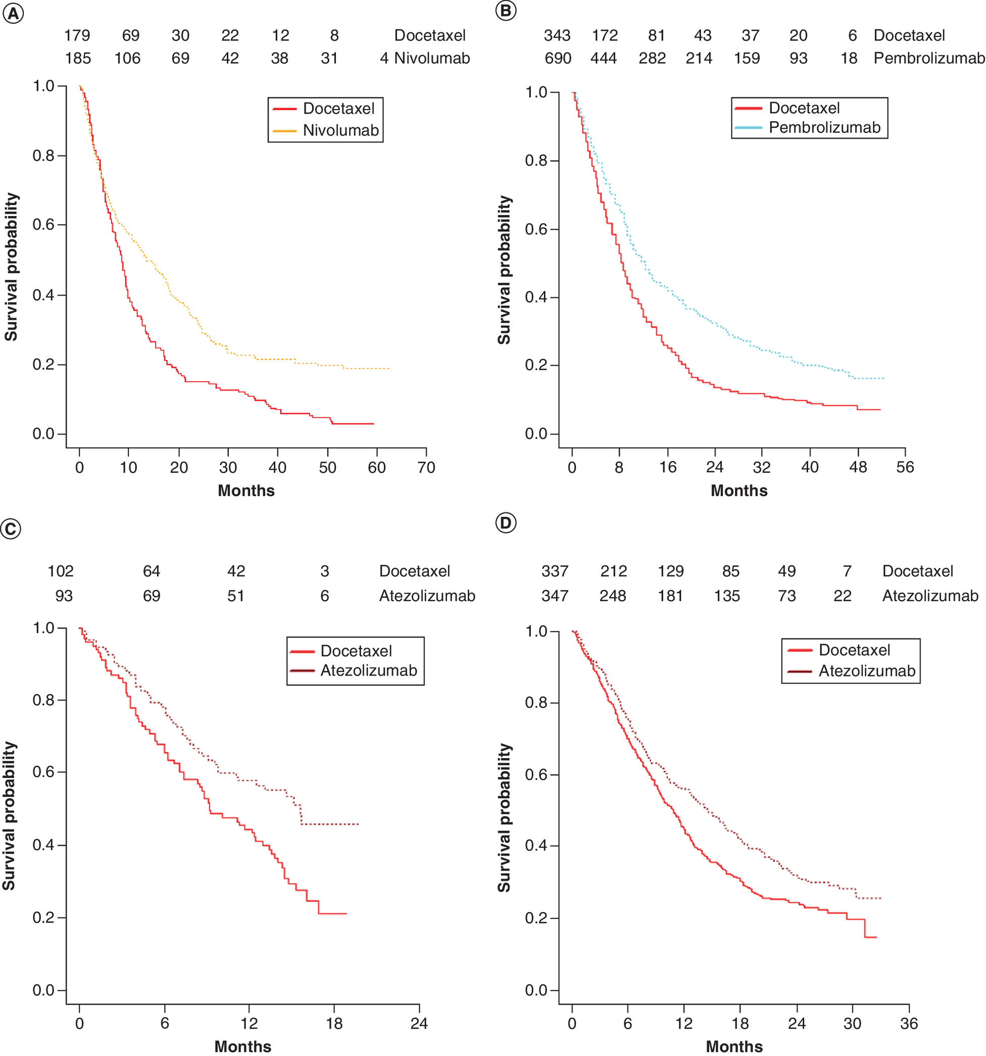
Figure 1. Reconstructed Kaplan–Meier curves in evidence network of overall survival.
(A) Pooled checkmate 017–057 trials comparing nivolumab with docetaxel. (B) Keynote 010 trial comparing pembrolizumab with docetaxel. (C) POPLAR trial comparing atezolizumab with docetaxel. (D) OAK trial comparing atezolizumab with docetaxel.
Statistical methodology
For all models described below, the corresponding equations are presented in Table 1. A fixed-effects model was preferred to a random-effects model, due to a limited network of evidence with only two trials comparing the same treatments. Placement of random effects is an issue for future research with numerous treatment effect parameters for which a random effect can be specified when considering flexible models. The pooled Checkmate 017 and 057 data set was used as reference trial for all NMA methodologies compared.
| Approach | Equations | Equations | Where | |
|---|---|---|---|---|
| 1 | PNMA Exponential Weibull Gompertz Log-normal Log-logistic | 2a 2b 2c 2d 2e 2f | S = survival all-cause mortality i = trial coefficient j = treatment coefficient t = time Sds = disease-specific survival Sgp = general population survival that is age and gender specific for the trials considered Reference therapy in the network is docetaxel. exp(α0i + α1j) = scale for study i and treatment j, where α0i is the log scale of the reference therapy for study i, and α1j codes for the treatment effect of treatment j vs reference therapy, α1 = 0 for the reference therapy exp(β0i + β1j) = shape for study i and treatment j, where β0i is the log shape of the reference therapy for study i, and β1j codes for the treatment effect of treatment j vs reference therapy, β1 = 0 for the reference therapy | |
| 2 | MCM NMA | 3 | γi = trial-specific effects on the log odds of cured patients γj = treatment-specific effects on the log odds of cured patients | |
| 3 | nMCM NMA | 4 | γi = trial-specific effects on the log odds of cured patients γj = treatment-specific effects on the log odds of cured patients | |
| 4 | PM-NMA | 5 | γi = trial-specific effects on the log odds of short-term surviving patients γj = treatment-specific effects on the log odds of short-term surviving patients S1 is the treatment and trial disease-specific survival for short-term surviving patients S2 is the treatment and trial disease-specific survival for long-term surviving patients | |
| 5 | FP-NMA | 6a 6b 6c 6d 6e 6f | c_h is the cumulative hazard h is the instantaneous hazard p1 and p2 are the powers of the fractional polynomial γ are the linear predictor coefficients of the fractional polynomial | |
| 6 | S-NMA | 7a 7b 7c 7d 7e | wlch = Weibull log cumulative hazard function s(t) ∼ spline function which in case of the Weibull concerns the log cumulative hazard kj = knot which is treated as a parameter and therefore estimated by the model; in this present example there is only one knot, so j = 1 kmin is minimum uncensored survival time kmax is maximum uncensored survival time γ are the linear predictor coefficients of the spline | |
| 7 | PW-NMA | For t in 0 to pwtp For t >= pwtp | 8a 8b 8c 8d | pwtp = piecewise time point, set to 2 years in this example S1 is the treatment and trial disease-specific survival before pwtp of 2 years S2 is the treatment and trial disease-specific survival after the pwtp of 2 years conditional on S1 exp(α10i + α11j) is for the first piece the scale for study i and treatment j exp(β10i + β11j) is for the first piece it is the shape for study i and treatment j exp(α20i + α21j) is the same as exp(α10i + α11j) but for second piece of the piecewise exp(β20i + β21j) is the same as exp(β10i + β11j) but for second piece of the piecewise |
FP-NMA: Fractional polynomial network meta-analysis; MCM NMA: Mixture cure model network meta-analysis; nMCM NMA: Non mixture cure model network meta-analysis; PM-NMA: Parametric mixture network meta-analysis; PNMA: Parametric network meta-analysis; PW-NMA: Piecewise network meta-analysis; S-NMA: Spline network meta-analysis.
Parametric NMA
The parametric NMA model assumes that the long-term survival of each treatment population in an evidence network follows one of the commonly used parametric distributions [2,24]. The parametric distribution functions were applied in the NMA setting as described by Equation 2 in Table 1, for which the parameters are written as the sum of study effect and treatment effect, thereby not breaking randomization.
Mixture & nonmixture cure NMA
The MCM NMA model assumes two separate patient groups: one relates to cured patients whose survival follows general population survival and the other relates to uncured patients whose survival is defined by a parametric distribution and general population survival [14]. This formalization is described by Equation 3 in Table 1.
The nMCM NMA model assumes that all patients belong to the same group, but that the event risk decreases to zero over time, meaning the entire cohort has a chance to be cured over time and only perish from general population mortality [15]. The survival function of the nMCM can be written as shown in Equation 4 in Table 1.
Parametric mixture NMA
The parametric mixture NMA model does not distinguish between cured and uncured patients but instead distinguishes between groups differing in survival. Parametric mixture NMAs estimate the TTE end point of distinct groups (latent subgroups such as short- and long-term survivors) based on separate parametric distributions. In this example, two distinct groups were defined (see Equation 5 in Table 1). A mixture of the same parametric distribution class with different parameters for long- and short-term survivors was used.
To ensure identifiability of the individual hazard components, the authors imposed an ordering constraint on the scale parameters, such that the scale parameter of distribution for the short-term survivors would have been smaller than the scale parameter of the long-term survivors. This is necessary because, with the same parameters, the individual components have identical likelihood contributions. The identifiability for the treatment effect is solved by relating the distribution for the shortest survival for the control arm to the distribution for the shortest survival for the active and analogously for the longest survival. Otherwise, the parameters might switch roles during the Markov Chain Monte Carlo simulation giving, for each parameter, posterior distributions that are a mixture over the supported values [38].
Fractional polynomial NMA
With the fractional polynomial NMA model, the instantaneous hazard over time is modeled. The hazards of the second-order fractional polynomials are presented in Equation 6c–f in Table 1. Fractional polynomials are extensions of standard parametric distributions, such as Weibull, Gompertz and exponential. For instance, if the two γ‘s (γ10i + γ11j) are zero in Equation 6d, the hazard function is identical to that of a Weibull. The second-order fractional polynomial includes power parameters p1 and p2. For these two power parameters, Sauerbrei et al. recommends using the following values: -2, -1, -0.5, 0, 0.5, 1, 2 and 3 to be tested, which results in 36 combinations of p1 and p2 [16]. Janssen et al. introduced NMAs based on fractional polynomials (FPs) [23]. For the purpose of this paper, instead of hard-coding p1 and p2 as suggested by Sauerbrei and Jansen et al., p1 and p2 were considered as model variables for which uniform prior distributions were specified between -3 and 3, with the condition that p1 is always smaller than p2. This reduces the number of FPs to four models: a first-order, second-order, repeated-power and logarithmic. This modification ensures that the optimal combination of p1 and p2 is estimated and that the number of settings for the FPs is reduced from 36 to 4 (Equation 6b–e in Table 1).
Modified spline NMA
Royston and Parmar proposed extending the Weibull, log-logistic and log-normal models to incorporate natural cubic splines based on the log cumulative hazard [17]. Spline-based models are flexible parametric models that are defined in stages by polynomial distributions intersected by ‘knots’ [17]. Beyond the final knot (kmax), the spline-cumulative hazard function follows the selected corresponding parametric distribution – that is, Weibull, log-logistic and log-normal. Besides splines on the log cumulative hazard, a spline based on the instantaneous hazard was used [39].
Royston and Parmar suggest placing the knot at the median of the log uncensored survival time when considering one knot; at 33rd and 66th percentile of the log uncensored survival times with two knots; and at the 25th, 50th and 75th percentiles with four knots. The times corresponding to these percentiles for the present data set are shown in Supplementary Table 1. The incremental times between knots is limited; for instance, 25% is 4 months and 75% is 14 months, given the exp(kmax) of 68 months, thereby limiting the added value of an extra knot. Therefore, the authors chose to focus on a one-knot model in the base case, with the knot placed at median uncensored survival of approximately log(8 months) for all trials in the evidence network. In a scenario analysis, they tested a two-knot Weibull spline and a one-knot Weibull spline with its knot at log(15 months) instead of log(8 months). The spline Equation 7 mentioned in Table 1 concerns the Weibull spline. Similar formulations are available for the log-normal, log-logistic splines and instantaneous hazards [17,39]. Equation 7a–e are similar to those reported by Royston and Parmar [17] with the exception that treatment- and trial-specific coefficients were added to allow for the splines to be used in a fixed-effects NMA framework. The authors extended the Royston/Parmer formulations to a Gompertz, given that the Gompertz is a log-Weibull distribution.
Piecewise parametric NMA
The piecewise parametric NMA approach uses conditional consecutive parametric distributions to estimate the TTE end point per period. For these analyses, the periods considered were before and after 8 months, consistent with the spline. In two scenario analyses, the authors considered a Weibull piecewise with pieces up to 8 months, between 8 and 12 months and beyond 12 months and a Weibull piecewise with periods before and after 15 months. The corresponding parametric distributions were applied in a fixed-effects NMA as described by Equation 8a–e (Table 1). Although the Weibull distribution is the focus in this formula, the same principle applies to other parametric distributions. Similar to mixture, for both pieces, the same parametric distribution was applied.
Statistical base case model selection & parametrization
In total, the authors tested 36 submodels based on seven model types: standard parametric, piecewise, spline, fractional polynomial, mixture and MCM and nMCM. Especially with more complex models, allowing for treatment coefficients on all parameters may result in an overfit and or extrapolations that are not optimal in terms of clinical plausibility. With 36 submodels and numerous possible treatment specification options per submodel in the NMA, a variable or treatment-effect selection parameter approach is needed. There are several somewhat complex Bayesian variable selection methods available, which are all related to goodness of fit of the observed data, rather than assessing clinically plausible extrapolation [40]. The authors chose a pragmatic two-step treatment-effect variable selection approach.
First, they ran 36 TTE submodels based on the seven models, for which they assigned treatment coefficients to all parameters. This is similar to the methodology described in the NICE Decision Support Unit TSD 21, which assumes individual models per treatment. In the second step, to avoid testing a large number of treatment-effect parameter specifications over the 36 tested models, per model, the distribution/specification with the lowest ‘leave-one-out’ information criterion (LOOIC) [41], best fit, was rerun, but only with treatment coefficients on those parameters for which the coefficient was larger than its corresponding standard deviation. Subsequently, of these seven ‘reduced’ models, the statistical base case model was selected based on the lowest LOOIC. The LOOIC serves the same purpose as the Akaike information criterion and can be seen as the Bayesian alternative for the frequentist Akaike information criterion, as demonstrated by Stone et al. [42].
General statistical approach
All conducted NMA approaches considered relative mortality. More specifically, they accounted for the UK general population mortality [43] in the likelihood function following the additive hazard approach suggested by Anderson et al. based on cubic splines and previously applied by Van Oostrum et al. on parametric distributions [44,45]. The present study used the UK life tables with mean age of 62 and gender distribution of 55% males based on Checkmate 017–057.
The tested NMA approaches were also compared based on LOOIC, mean and incremental mean survival and corresponding uncertainty (defined as the width of the 95% credible intervals of the mean and incremental mean survival).
Also, a potential decision flow diagram for TTE NMAs informing cost–effectiveness models is proposed.
All TTE end point NMAs were performed using the RStan package in R Statistical Software (version 1.2.0) [46]. These analyses were fitted with weakly informative priors [47]. For all modeled parameters, the authors applied normal priors with a mean of 0 and a standard deviation of 5. This was with the exception of the following parameters of more flexible models, where smaller standard deviations were applied to improve convergence: The standard deviation of the treatment effect on the third spline parameter was set to 0.1. The standard deviations of the baseline and treatment effect of the two shape parameters of the mixture were set to 0.5 and the standard deviations of the distribution parameter (γ) and the corresponding treatment effects were set to 1.
The models were run with three chains of 10,000 iterations, of which 5000 were burn-in iterations to generate the posteriors for the defined parameters. Convergence of the three chains was tested using the Rhat test, as introduced by Gelman and Rubin [48].
Results
Among the four trials in the present evidence network, the proportional hazard (PH) assumption on OS was violated for pooled Checkmate 017–057 studies but not for the other trials (see Supplementary Figure 3).
Table 2 shows the LOOICs for the best-fitting distributions/setting per flexible survival model type tested. The log-logistic piecewise model had the lowest LOOIC, with 13,434. It also shows the parametrization of the reduced models with best-fitting distributions and corresponding LOOICs, which are typically lower. Of the reduced models, the piecewise log-logistic model also had the best LOOIC.
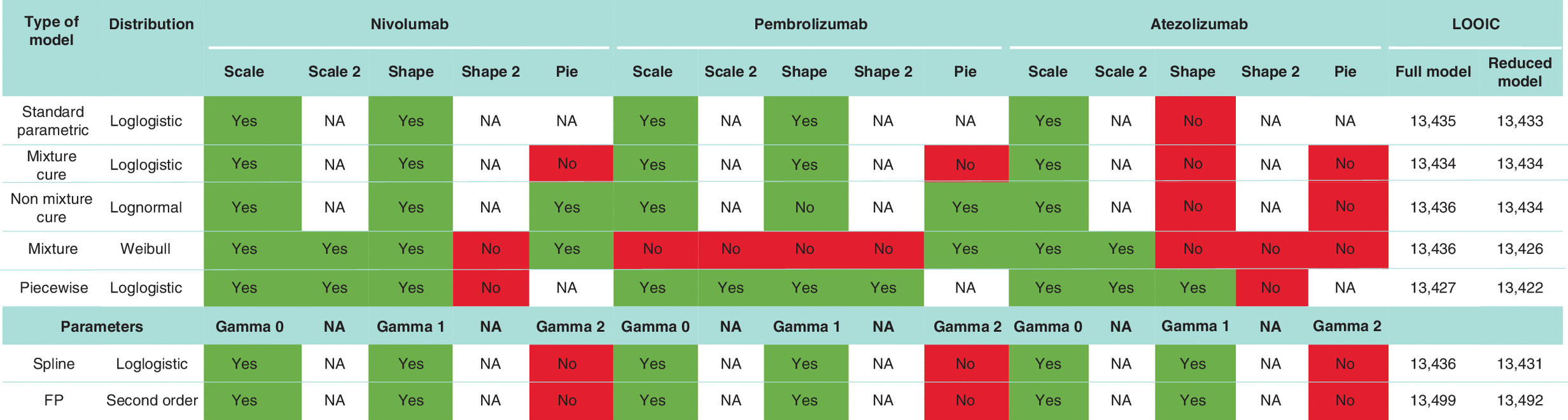 |
FP: Fractional polynomial; NA: Not available.
Figure 2 shows the mean incremental survival for nivolumab, pembrolizumab and atezolizumab compared with docetaxel, as well as the corresponding uncertainty defined as the range of the 95% credible interval for both the full and reduced models. Compared with the standard parametric NMA, which is the least complex model with the lowest number of variables, flexible models impact the incremental mean survival and increase the corresponding uncertainty. In the fully specified log-logistic parametric NMA, the incremental survival compared with docetaxel was 1.73, 1.04 and 0.57 for nivolumab, pembrolizumab and atezolizumab, respectively. The corresponding numbers for the Weibull mixture model, which is the most flexible model with the most variables, were 3.14, 0.47 and 2.99, respectively. In terms of uncertainty, the fully specified log-logistic parametric NMA showed an uncertainty range for the incremental survival 1.69, 1.11 and 1.00, respectively. The corresponding numbers for the Weibull mixture model were 3.76, 2.55 and 10.00, respectively.
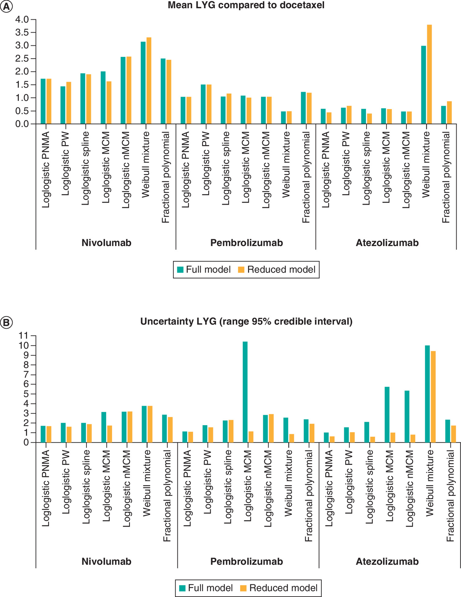
Figure 2. Incremental results of nivolumab, pembrolizumab and atezolizumab all compared to docetaxel of best-fitting distributions per full and reduced model.
(A) An overview of mean incremental survival. (B) An overview of corresponding uncertainty, defined as the range of the 95% credible interval of mean incremental survival.
LYG: Life years gained; MCM: Mixture cure model; nMCM: Nonmixture cure model; PNMA: Parametric network meta-analysis; PW: Piecewise.
The treatment-effect parametrization reduction method also seems to impact incremental survival, reducing uncertainty over the incremental mean survival. In the reduced log-logistic parametric NMA, incremental survival for nivolumab, pembrolizumab and atezolizumab compared with docetaxel was 1.73, 1.04 and 0.44, respectively. The corresponding numbers for the Weibull mixture model were 3.31, 0.49 and 3.80, respectively. In terms of uncertainty, the fully specified log-logistic parametric NMA showed an uncertainty range for incremental survival of 1.66, 1.09 and 0.62, respectively. The corresponding numbers for the Weibull mixture model were 3.77, 0.85 and 9.42, respectively. The predicted OS rates for the reduced models are presented in Supplementary Figure 4.
The scenario analyses on the spline Weibull showed that the LOOIC slightly improved from 13,440 with one knot to 13,438 with two knots and 13,435 with the one knot placed at 75th percentile of the log uncensored survival time. The corresponding analyses with the piecewise Weibull showed that the LOOIC worsened from 13,454 in the base case to 13,846 with three pieces and 13,480 with pieces before and after 15 months instead of 8 months.
Figure 3 shows a potential decision flow diagram for TTE comparative effectiveness survival extrapolations approaches informing cost–effectiveness models. For the present evidence network, pseudo individual patient-level data could be derived from published KM curves for all studies. For Checkmate, the Weibull mixture cure resulted in estimated cure rates of 0.02 (0.00– 0.06) for docetaxel and 0.18 (0.11–0.25) for nivolumab. Whether cure is truly clinical plausible for a subset of patients in advanced non-small-cell lung cancer PD-L1 >1% or whether there is a subset of patients that could be considered long-term survivors, but not cured, is an important clinical question. If clinicians or other medical experts expect that part of the population will be instantaneously cured, the mixture cure model is preferred. If clinicians or other medical experts believe there is no population that is instantaneously cured, but once people have survived a number of years, the disease-related event probability is negligible, a nMCM is preferred. If clinicians indicate that there is just a difference in latent groups of short- and long-term survivors, the mixture NMA approach is preferred over the mixture cure models. One could alternatively consider multiple latent groups instead of only short- and long-term survivors and when individual patient data of all trials are available (not typically being the case) differences between manifest groups can also be modeled using covariates. If clinicians do not believe in a subset of long-term survivors and the standard parametric models fit well, the standard parametric NMA is preferred. Finally, if the standard parametric NMA provides suboptimal fit and or clinically implausible extrapolations, the spline, piecewise or FP approaches can be considered.
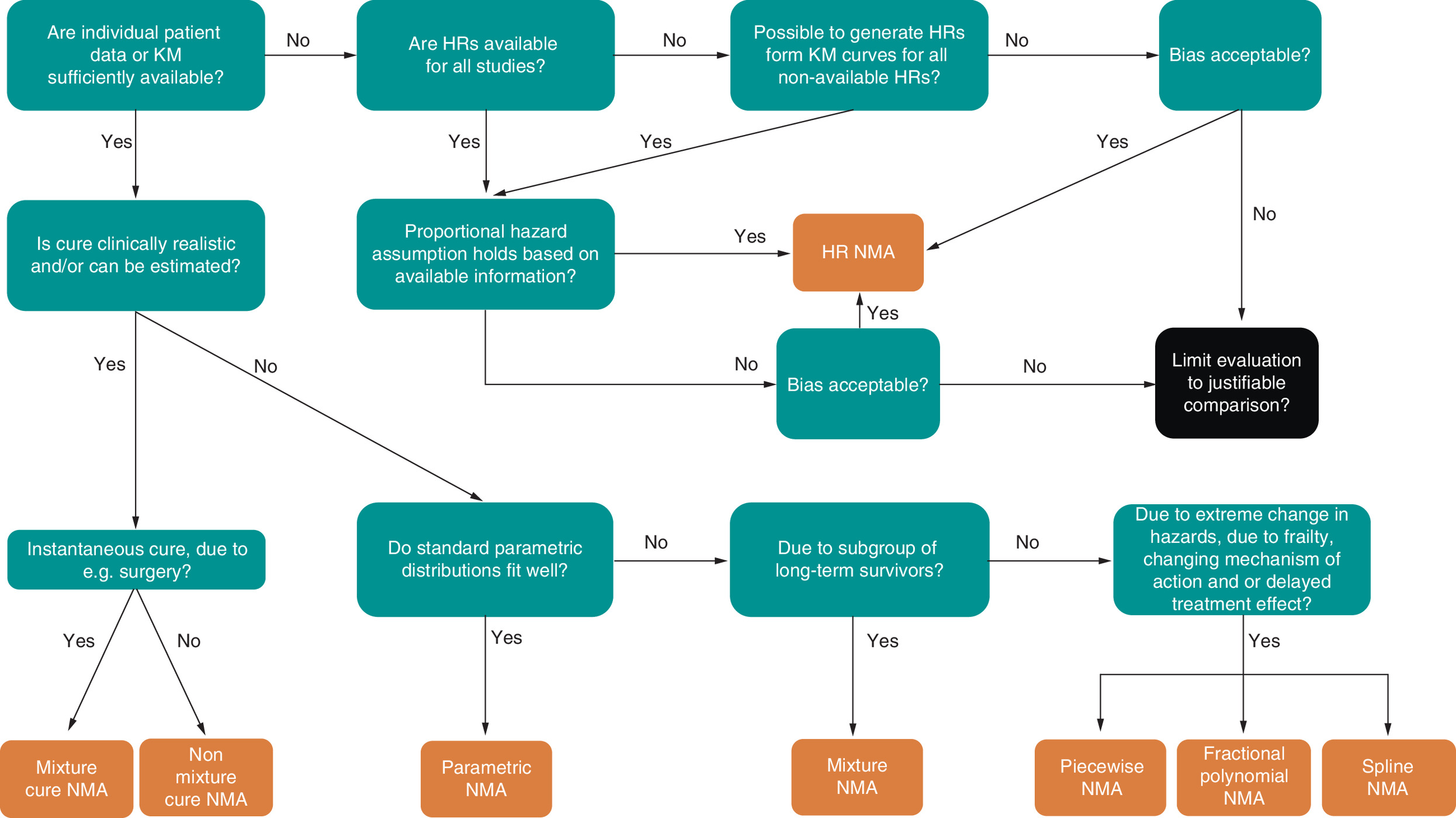
Figure 3. Flow diagram for selection time-to-event network meta-analysis approach.
HR: Hazard ratio; KM: Kaplan Meir; NMA: Network meta-analysis.
Discussion
This paper presents the generalization of the existing trial-based flexible model extrapolation techniques to the NMA space while considering excess mortality and selection of base case model, distribution and optimal treatment-effect parametrization.
Compared with the standard parametric NMA, flexible models impact the incremental mean survival and increase the corresponding uncertainty. The treatment-effect parametrization reduction method also seems to impact incremental survival, reduce uncertainty over the incremental mean survival and generally improve the fit statistic in terms of LOOIC.
Each discussed NMA method is not without strengths or limitations. A strength of all methods explored in this paper is that they do not rely on the PH assumption. A downside to these flexible TTE NMA approaches is the need for individual patient data or published KM curves, which might not always be in the public domain. Regarding the present network, relatively mature survival data were available for pembrolizumab and nivolumab, compared with relatively immature survival data for atezolizumab for the considered PD-L1 >1% subpopulations in the OAK and POPLAR trials. Dealing with immature data for a certain treatment is complex and constitutes a general limitation of survival extrapolations, which is not limited to the context of NMA and flexible models. The impact of this limitation is evident in the heterogenous results observed for atezolizumab, in terms of both incremental mean survival and corresponding uncertainty, which was 0.44 with uncertainty range of 0.62 years for standard log-logistic NMA versus 3.80 and 9.44 years for the mixture Weibull NMA. A solution in an NMA setting could be to consider class treatment effects, allowing in this case a comparison between docetaxel and immuno-oncology therapies, but not among the immuno-oncology therapies. Another solution requiring less rigorous assumptions would be Bayesian hierarchical modeling, as suggested by Schoenfeld, allowing for the borrowing of information across mature and immature trials for parameter estimation in the flexible model NMAs [49]. Alternatively, one can use other prior data in a Bayesian perspective. For instance, for MCMs and nMCMs the cure parameter could be informed by fitting these models on the progression-free survival data, which are typically more mature than OS and assume that the OS cure rate should be at least as high as the progression-free survival cure rate.
Besides the immaturity of underlying data, a limitation of MCMs and nMCMs in an NMA setting is that in cases where the cure is estimable for the active treatment but not for the reference placebo treatment, the treatment effect on cure for that active treatment becomes very large. Applying that treatment effect to another reference trial in the NMA where cure was estimable for the reference treatment is likely to substantially inflate the cure rate for that active treatment. A limitation of the Gompertz model for MCM and nMCMs is that the shape parameter of the Gompertz can be negative, so that, on its own, it predicts a percentage of patients never experiencing an event. This implies that the estimated percentage of patients never obtaining an event for the Gompertz cure models is partly modeled by the Gompertz and partly by the cure parameter.
The parametric mixture NMA approach is very flexible, as it can combine different parametric distributions over the fractions (e.g., Weibull for fraction 1 and log-normal for fraction 2) as well as use several fractions (e.g., short, intermediate, long survivors) and treatment effects can be placed on all parameters. It is less restrictive in its use than nMCMs and MCMs, as it does not require that cure is clinically plausible in the indication. A limitation of the parametric mixture is that the number of estimable parameters is high, which is likely to explain the substantial uncertainty over the atezolizumab mean survival.
FP-NMAs allow dramatic changes in hazards over time. The complex functional forms of the FPs mean that it is harder to link the behavior of the function to clinical background information. The authors reduced the required number of FPs to be tested from 36 to 8 by defining p1 and p2 as parameters [23]. Similar to Janssen et al., the paper focused on second-order FPs; first-order FPs were not assessed [23].
Spline NMAs are flexible, which is an advantage compared with standard parametric curve in data sets with more extreme changes in hazards over time. However, like FPs, their complex functional forms make it harder to interpret the function from a clinical perspective and their extrapolations can vary massively. Royston and Parmar recommend placing the knot on the median uncensored survival of the trial. Dias et al. mention that knots should be placed at the same time points within an NMA framework [50]. For this paper, only splines with one knot were considered, as additional knots do not seem to improve the fit generally [17]. Spline NMAs with multiple knots can obviously be defined.
A limitation of piecewise models is that due to the pieces, more discontinuous changes of hazards may be modeled. Discontinuous hazards are typically clinically implausible for pharmaceutical treatments. Another limitation is that the time points for the pieces and the number of pieces are subjective and many options can be tested for statistical and clinical plausibility. For this paper, the data were divided into prior and beyond 1 year. Other time points could have changed the results of the piecewise models. For both the spline and piecewise NMA, it is important to consider the number and placement of knots, as they impacted the fit and might improve further in other NMA data sets.
A standard NMA method for TTE data is the pooling of hazard ratios, which was not assessed in the present paper due to violation of the PH assumption in the nivolumab trial. Moreover, hazard ratios are typically reported for all-cause mortality in clinical trials. As suggested by NICE Decision Support Unit TSD 21 [1], the authors considered relative survival. Combining an all-cause mortality hazard ratio with disease-specific mortality parametric survival prediction should only be done when the impact of general population mortality during observation period trials is negligible.
The authors used a pragmatic two-step approach to select the optimal model, corresponding distribution/setting and treatment-effect specification, given the evidence network. In future research, formal Bayesian variable selection methods [40] may be considered. However, those and this pragmatic two-stage method focus on optimal fit over the considered trial periods. The trial period is not the primary interest, as the authors already have the KM data for this period. More important is the clinical plausibility of the extrapolations, which needs to be validated with external long-term data and justified expert opinion. Also, the optimal model in terms of fit might not be the best-fitting model for the pivotal trial of interest in the evidence network, so visual inspection of the fit and extrapolation for the reference trial remains important.
Conclusion
In conclusion, the authors extended the following flexible trial-based extrapolation models to a relative survival NMA framework: mixture, MCM, nMCM and piecewise NMAs. The authors also introduced the Gompertz spline, which was not yet available for individual trial analyses and the NMA framework. This is important, as the same extrapolation techniques for individual trials should be available in the NMA setting to ensure that the most clinically plausible extrapolations are selected for health technology assessment.
Future perspective
In future research, combining these methods with multilevel NMAs to adjust for effect modification might be needed when distribution of effect modifiers is heterogenous over trials in the network [51]. One might also consider mixing models, such as a spline MCM, a piecewise MCM or an FP mixture model. The possibilities are almost infinite. Choice and placement of random effects on distributions like the mixture Weibull, which would allow for up to five random effects, are also apt for future research. In future research, it will be important to compare the FP approach in which p1 and p2 are defined as variables instead of as values with the FP approach by Jansen et al., who define p1 and p2 as values. To assess the validity of the predicted survival extrapolations per the presented NMA approach, it will be important in the future to conduct simulation studies assessing the validity of the survival extrapolations for the treatments in the evidence network. This requires extensive simulations, as different models might be better at different evidence network data sets. The following data set simulation variables may be considered: number of trials, maturity, sample size and impact of treatment (e.g., PH and cure or long-term survival for one or more treatments in the evidence network).
•
Cost–effectiveness evaluations often rely on extrapolation techniques to calculate mean survival, incremental mean survival and their corresponding uncertainties.
•
Health authorities provide guidance on appropriate standard parametric extrapolation techniques for individual trials.
•
NICE Decision Support Unit Technical Support Document 21 focuses on flexible survival models and the concept of modeling excess or relative mortality in individual trials, as standard parametric approaches might not provide optimal trial extrapolations for all treatments and/or diseases.
•
In trial-based extrapolations, parametric distributions, splines, piecewise models, mixture and nonmixture cure and parametric mixture models have been explored.
•
Standard parametric distributions, but also flexible methods such as splines and fractional polynomials, have been introduced in the network meta-analysis (NMA) setting to compare several regimens simultaneously across various networks of studies where the proportional hazards assumption may be violated.
•
The authors extended the following flexible, trial-based extrapolation models to a relative survival NMA framework and conducted mixture, mixture cure and non-mixture cure models, and piecewise NMAs.
•
The authors also introduced the Gompertz spline, which was not yet available for individual trial analyses and the NMA framework.
•
The same extrapolation techniques for individual trials should be available in the NMA setting to ensure that the most clinically plausible extrapolations are selected for health technology assessment submission.
Financial & competing interests disclosure
B Heeg, I van Oostrum, A Garcia, S van Beekhuizen and A Verhoek are employees of Cytel, which is a consulting company for pharmaceutical companies. Cytel did not receive grants or honoraria related to this research. JC Cappelleri and S Roychoudhury are employees of Pfizer. MJ Postma received various grants and honoraria, all unrelated to this research. MJNM Ouwens is an employee of AstraZeneca. The authors have no other relevant affiliations or financial involvement with any organization or entity with a financial interest in or financial conflict with the subject matter or materials discussed in the manuscript apart from those disclosed.
No writing assistance was utilized in the production of this manuscript.
Open access
This work is licensed under the Attribution-NonCommercial-NoDerivatives 4.0 Unported License. To view a copy of this license, visit http://creativecommons.org/licenses/by-nc-nd/4.0/
Supplementary Material
References
1.
NICE DSU Technical Support Document 2: A Generalised Linear Modelling Framework for Pairwise and Network Meta-analysis of Randomised Controlled Trials. NICE, London, UK (2011).
2.
NICE DSU Technical Support Document 14: Survival Analysis for Economic Evaluations alongside Clinical Trials – Extrapolation with Patient-Level Data. NICE, London, UK (2011).
3.
Guidelines for the Economic Evaluation of Health Technologies: Canada. Canadian Agency for Drugs and Technologies in Health. Ottowa, Canada (2017).
4.
Guidelines for Preparing Submissions to the Pharmaceutical Benefits Advisory Committee (PBAC). Version 5.0, September 2016. Department of Health, Canberra Australia (2016).
5.
Technology Appraisal Guidance [TA517] – Avelumab for Treating Metastatic Merkel Cell Carcinoma. NICE, London, UK (2021).
6.
Technology Appraisal Guidance [TA519] – Pembrolizumab for Treating Locally Advanced or Metastatic Urothelial Carcinoma after Platinum-Containing Chemotherapy. NICE, London, UK (2018).
7.
Technology Appraisal Guidance [TA520] – Atezolizumab for Treating Locally Advanced or Metastatic Non-small-cell Lung Cancer after Chemotherapy. NICE, London, UK (2018).
8.
Technology Appraisal Guidance [TA531] – Pembrolizumab for Untreated PD-L1-Positive Metastatic Non-small-cell Lung Cancer NICE, London, UK (2018).
9.
Technology Appraisal Guidance [TA554] – Tisagenlecleucel for Treating Relapsed or Refractory B-cell Acute Lymphoblastic Leukaemia in People Aged Up to 25 Years. NICE, London, UK (2018).
10.
Technology Appraisal Guidance [TA545] – Gemtuzumab Ozogamicin for Untreated Acute Myeloid Leukaemia. NICE, London, UK (2018).
11.
Technology Appraisal Guidance [TA589] – Blinatumomab for Treating Acute Lymphoblastic Leukaemia in Remission with Minimal Residual Disease Activity. NICE, London, UK (2019).
12.
Technology Appraisal Guidance [TA559] – Axicabtagene Ciloleucel for Treating Diffuse Large B-cell Lymphoma and Primary Mediastinal Large B-cell Lymphoma after 2 or More Systemic Therapies. NICE, London, UK (2019).
13.
Technology Appraisal Guidance [TA552] – Liposomal Cytarabine-Daunorubicin for Untreated Acute Myeloid Leukaemia. NICE, London, UK (2018).
14.
Lambert PC, Thompson JR, Weston CL, Dickman PW. Estimating and modeling the cure fraction in population-based cancer survival analysis. Biostatistics 8(3), 576–594 (2006).
15.
Swain PK, Grover G, Goel K. Mixture and non-mixture cure fraction models based on generalized Gompertz distribution under Bayesian approach. Tatra Mt. 66(1), 121–135 (2016).
16.
Sauerbrei W, Royston P, Look M. A new proposal for multivariable modelling of time-varying effects in survival data based on fractional polynomial time-transformation. Biomet. J. 49(3), 453–473 (2007).
17.
Royston P, Parmar MKB. Flexible parametric proportional-hazards and proportional-odds models for censored survival data, with application to prognostic modelling and estimation of treatment effects. Stat. Med. 21(15), 2175–2197 (2002).
18.
Ducros F, Pamphile P. Bayesian estimation of Weibull mixture in heavily censored data setting. Reliabil. Eng. Syst. Saf. 180, 453–462 (2018).
19.
Mohammed YA, Yatim B, Ismail S. A simulation study of a parametric mixture model of three different distributions to analyze heterogeneous survival data. Modern App. Sci. 7(7), 1–9 (2013).
20.
Ouwens MJNM, Mukhopadhyay P, Zhang Y, Huang M, Latimer N, Briggs A. Estimating lifetime benefits associated with immuno-oncology therapies: challenges and approaches for overall survival extrapolations. Pharmacoeconomics 37(9), 1129–1138 (2019).
21.
Cislo PR, Emir B, Cabrera J, Li B, Alemayehu D. Finite mixture models, a flexible alternative to standard modeling techniques for extrapolated mean survival times needed for cost–effectiveness analyses. Value Health 24(11), 1643–1650 (2021).
22.
NICE DSU Technical Support Document 21. Flexible Methods for Survival Analysis. NICE, London, UK (2020).
23.
Jansen JP. Network meta-analysis of survival data with fractional polynomials. BMC Med. Res. Methodol. 11(1), 61 (2011).
24.
Ouwens MJNM, Philips Z, Jansen JP. Network meta-analysis of parametric survival curves. Res. Synth. Methods 1(3–4), 258–271 (2010).
25.
Freeman SC, Carpenter JR. Bayesian one-step IPD network meta-analysis of time-to-event data using Royston-Parmar models. Res. Synth. Methods 8(4), 451–464 (2017).
26.
Astrazeneca. National Institute for Health and Care Excellence (NICE). Technology Appraisal Guidance [TA503] – Fulvestrant for Untreated Locally Advanced or Metastatic Oestrogen-Receptor Positive Breast Cancer NICE, London, UK (2018).
27.
Wiecek W, Karcher H. Nivolumab versus cabozantinib: comparing overall survival in metastatic renal cell carcinoma. PLOS ONE 11(6), 1–11 (2016).
28.
Cope S, Jansen JP. Quantitative summaries of treatment effect estimates obtained with network meta-analysis of survival curves to inform decision-making. BMC Med. Res. Methodol. 13, 1–11 (2013).
29.
Cope S, Ouwens MJNM, Jansen JP, Schmid P. Progression-free survival with fulvestrant 500 mg and alternative endocrine therapies as second-line treatment for advanced breast cancer: a network meta-analysis with parametric survival models. Value Health 16(2), 403–417 (2013).
30.
Kim J, Cho J, Lee MH, Lim JH. Relative efficacy of checkpoint inhibitors for advanced NSCLC according to programmed death-ligand-1 expression: a systematic review and network meta-analysis. Sci. Rep. 8(1), 1–8 (2018).
31.
Borghaei H, Gettinger S, Vokes EE et al. Five-year outcomes from the randomized, phase III trials CheckMate 017 and 057: nivolumab versus docetaxel in previously treated non-small-cell lung cancer. J. Clin. Oncol. 39(7), 723–733 (2021).
32.
Herbst RS, Garon EB, Kim DW et al. Long-term outcomes and retreatment among patients with previously treated, programmed death-ligand 1-positive, advanced non-small-cell lung cancer in the KEYNOTE-010 study. J. Clin. Oncol. 38(14), 1580–1590 (2020).
33.
Fehrenbacher L, Von Pawel J, Park K et al. Updated efficacy analysis including secondary population results for OAK: a randomized phase III study of atezolizumab versus docetaxel in patients with previously treated advanced non-small cell lung cancer. J. Thorac. Oncol. 13(8), 1156–1170 (2018).
34.
Fehrenbacher L, Spira A, Ballinger M et al. Atezolizumab versus docetaxel for patients with previously treated non-small-cell lung cancer (POPLAR): a multicentre, open-label, phase 2 randomised controlled trial. Lancet 387(10030), 1837–1846 (2016).
35.
Rittmeyer A, Barlesi F, Waterkamp D et al. Atezolizumab versus docetaxel in patients with previously treated non-small-cell lung cancer (OAK): a phase 3, open-label, multicentre randomised controlled trial. Lancet 389(10066), 255–265 (2017).
36.
Mitchell M, Muftakhidinov B, Winchen T. Engauge digitizer software (2020). https://markummitchell.github.io/engauge-digitizer/
37.
Guyot P, Ades AE, Ouwens MJNM, Welton NJ. Enhanced secondary analysis of survival data: reconstructing the data from published Kaplan–Meier survival curves. BMC Med. Res. Methodol. 12(1), 9 (2012).
38.
Demiris N, Lunn D, Sharples LD. Survival extrapolation using the poly-Weibull model. Stat. Methods Med. Res. 24(2), 287–301 (2015).
39.
Crowther MJ, Lambert PC. stgenreg: a Stata package for general parametric survival analysis. J. Stat. Software 53(12), 1–17 (2013).
40.
O'Hara B, Sillanpää M. A review of Bayesian variable selection methods: what, how and which. Bayesian Analysis 4, 85–117 (2009).
41.
Vehtari A, Gelman A, Gabry J. Practical Bayesian model evaluation using leave-one-out cross-validation and WAIC. Stat. Comput. 27(5), 1413–1432 (2017).
42.
Stone M. An asymptotic equivalence of choice of model by cross-validation and Akaike's criterion. J. Royal Stat. Soc. B 39(1), 44–47 (1977).
43.
National life tables, UK: 2016 to 2018. www.ons.gov.uk/releases/nationallifetablesuk2016to2018
44.
Andersson TML, Dickman PW, Eloranta S, Lambe M, Lambert PC. Estimating the loss in expectation of life due to cancer using flexible parametric survival models. Stat. Med. 32(30), 5286–5300 (2013).
45.
Van Oostrum I, Ouwens M, Remiro-Azócar A et al. Comparison of parametric survival extrapolation approaches incorporating general population mortality for adequate health technology assessment of new oncology drugs. Value Health 24(9), 1294–1301 (2021).
46.
rstan®, package insert. Available at: https://cran.r-project.org/web/packages/rstan/rstan.pdf.
47.
Betancourt M. How the Shape of a Weakly Informative Prior Affects Inferences. R package version 2(1), (2017). https://mc-stan.org/users/documentation/case-studies/weakly_informative_shapes.html
48.
Gelman A, Rubin DB. Inference from iterative simulation using multiple sequences. Statist. Sci. 7(4), 457–472 (1992).
49.
Schoenfeld DA, Hui Z, Finkelstein DM. Bayesian design using adult data to augment pediatric trials. Clin. Trials 6(4), 297–304 (2009).
50.
Dias S, Ades AE, Welton NJ, Jansen JP, Sutton AJ. Network Meta-analysis for Decision-Making. John Wiley & Sons, Hoboken, NJ, USA (2018).
51.
Phillippo DM, Dias S, Ades AE et al. Multilevel network meta-regression for population-adjusted treatment comparisons. J. Royal Stat. Soc. Ser. A Stat. Soc. 183(3), 1189–1210 (2020).
Information & Authors
Information
Published In
Copyright
© 2022 Cytel. This work is licensed under the Attribution-NonCommercial-NoDerivatives 4.0 Unported License
History
Received: 28 February 2022
Accepted: 8 August 2022
Published online: 12 September 2022
Keywords:
Topics
Authors
Metrics & Citations
Metrics
Article Usage
Article usage data only available from February 2023. Historical article usage data, showing the number of article downloads, is available upon request.
Citations
How to Cite
Novel and existing flexible survival methods for network meta-analyses. (2022) Journal of Comparative Effectiveness Research. DOI: 10.2217/cer-2022-0044
Export citation
Select the citation format you wish to export for this article or chapter.
Citing Literature
- Andre Verhoek, Mario JNM Ouwens, Bart Heeg, Frank GA Jansman, Maarten J Postma, Simplifying fractional polynomials in Bayesian network meta-analysis via variable powers, Journal of Comparative Effectiveness Research, 10.57264/cer-2025-0126, 15, 1, (2025).
- Keith Chan, Sarah Goring, Kabirraaj Toor, Murat Kurt, Andriy Moshyk, Jeroen Jansen, Incorporating the possibility of cure into network meta-analyses: A case study from resected Stage III/IV melanoma, Research Synthesis Methods, 10.1017/rsm.2025.10038, 17, 1, (157-169), (2025).
- Taihang Shao, Mingye Zhao, Fenghao Shi, Mingjun Rui, Wenxi Tang, NMAsurv: An R Shiny application for network meta-analysis based on survival data, Research Synthesis Methods, 10.1017/rsm.2025.10020, 16, 6, (1042-1056), (2025).
- Bart Heeg, Dawn Lee, Jane Adam, Maarten Postma, Mario Ouwens, Defining Biological and Clinical Plausibility: The DICSA Framework for Protocolized Assessment in Survival Extrapolations Across Therapeutic Areas, PharmacoEconomics, 10.1007/s40273-025-01485-0, 43, 7, (793-803), (2025).
- Christopher G. Fawsitt, Janice Pan, Philip Orishaba, Christopher H. Jackson, Howard Thom, Unanchored simulated treatment comparison on survival outcomes using parametric and Royston-Parmar models with application to lenvatinib plus pembrolizumab in renal cell carcinoma, BMC Medical Research Methodology, 10.1186/s12874-025-02480-x, 25, 1, (2025).
- Suzanne C. Freeman, Alex J. Sutton, Nicola J. Cooper, Alessandro Gasparini, Michael J. Crowther, Neil Hawkins, Bayesian pairwise meta‐analysis of time‐to‐event outcomes in the presence of non‐proportional hazards: A simulation study of flexible parametric, piecewise exponential and fractional polynomial models, Research Synthesis Methods, 10.1002/jrsm.1722, 15, 5, (780-801), (2024).