Conditional power for assessing population interventions
Abstract
Aim: To calculate conditional power in comparative two-period studies with previously observed baseline data. Method: Isolate the variability attributable to the yet-to-observed data and modify the standard power formulae. Results: For illustration, we examine rates of opioid overdose before and after a reformulation of one opioid product. The null hypothesis posited no impact of the reformulation, alternative hypotheses posited possible impacts, and ancillary hypotheses posited different secular pre-post changes directly observable in comparators. Conditional power varied with the size of the comparator population and with the assumed pre-post change for the comparator. Conclusion: Pre-post designs can be initiated after the baseline period is over. Power calculations that are conditioned on observed baseline data account differently for variability in the baseline and follow-up periods.
For two-period comparative effectiveness analyses when baseline data already exist, it is valuable to know in advance if the study will have enough power to detect a meaningful difference. This scenario occurs in evaluating a reformulation of a medicinal product and in assessing the impact of public health or safety interventions (e.g., risk evaluation and mitigation strategies) [1]. The change in incidence of an outcome after the intervention will depend on the effectiveness of the intervention to reduce the rate of occurrence of the outcome and on secular trends.
The ratio of rate ratios (ROR) is a measure that compares pre- to post-intervention changes in a test product versus comparators to which the intervention in question does not apply. The logarithm of the ROR is the ‘difference-in-differences’ for the logarithms of the four component rates [2]. The ROR can be used as a measure of the impact of the intervention. We know of no published methods for calculating power of the pre-post two-product design for the common setting in which baseline data are in hand at study start.
The goal of this paper is to provide an accessible method and example R code for calculating the probability that a two-group intervention-assessment study will reject the null hypothesis of no effect of the intervention when only the post-intervention data are left to be collected.
The development presented here arose from an evaluation requested by the US FDA to assess the change in incidence of opioid overdose (OOD) in users of the opioid OxyContin (referred to hereafter as the ‘test product’) before and after it was reformulated to deter crushing and dissolution of the tablets. The FDA request was for a difference-in-differences design in very large health insurance database. (See Peacock and colleagues [3] for a general review of study designs to evaluate the effects of abuse deterrent formulations of opioid products.) Comparators specified by the FDA were other opioid products with similar indications but which had no change in their product formulation. The need was for power calculations that accommodated the already accrued parts of the comparison. An important aspect of this motivating example is that there were many potential comparators for the test product. The choice among them would have to be driven in part by questions of feasibility – would there be enough data to have a good chance at obtaining an actionable result? There remained moreover the possibility that none of the available comparators would be sufficient in the available data, so that further resources (databases) would need to be recruited.
With some data already known, the probability of future significant outcomes is the conditional power, defined as “the probability that the final study result will be statistically significant, given the data observed thus far and a specific assumption about the pattern of the data to be observed in the remainder of the study …” [4] For clinical trials, Lan and Wittes and others developed the idea of conditional power into curtailed testing (early decision-making when an outcome has become inevitable) and stochastic curtailment (early decision-making when an outcome is sufficiently probable) [5–8]. Conditional power calculations are also linked to procedures for determining futility in group sequential designs, and they have been advocated when unplanned interim analyses may be required in observational studies [9,10].
Standard power calculations for comparative change analyses assume that the observations become available only after the analysis plan has been finalized, so that the probability distributions of the measure under different scenarios are the same as those used to create a test statistic [11,12]. By analogy to the setting of a partly finished study, the present development instead analyzes the conditional power at the time when the number of events in test product users and comparators is already approximately known for the period before an intervention, and when the person-time of exposure is known or estimable for both the pre- and post-intervention periods. The number of events in test product and comparator users will happen in the future or is unknown and depends on the effectiveness of the intervention in reducing events (e.g., does reformulation of opioid products to forms that are difficult to crush or dissolve reduce overdoses in opioid users?). This was the data configuration available to us at the time we developed the method described here.
Data
The given data were: the numbers of events and the person-time of exposure in the pre-intervention period for the test product and during the corresponding calendar time for comparators; the expected amounts of person-time available for the test product and comparators in the post-reformulation period, based on preliminary data.
The development below treats counts of events as realizations of independent Poisson processes, with means equal to the period-by-product-specific event rates multiplied by the corresponding amounts of person-time. Application of the methods to settings with anticipated Poisson over-dispersion would require proportionately larger samples, but would otherwise be similar. The data consist of tabular summaries without personal identifiers. No ethical review was sought. We do not elaborate on the substantive questions raised by the example, including of the medical suitability of different comparator drugs, the necessity for covariate control or the choice of timing.
The ROR in Poisson regression
The final analysis of the predictors of rates will generally be accomplished by Poisson regression. The regression parameters will be estimated using a saturated model consisting of main-effect terms for drug (test vs comparator) and period (post- vs pre-intervention), in addition to a term for the drug–period interaction. The interaction term, which equals the logarithm of the estimated ROR, is the difference-in-differences measure.
The nonstandard aspect of the required power calculation is that the future variability resides uniquely in the post-reformulation event counts. The consequence is that a variance based on a full scenario of pre- and post-intervention expected counts will lead to overestimation of the uncertainty of future outcomes, and so cannot be used for power calculations.
Variance of estimates of the ROR
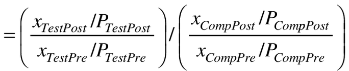
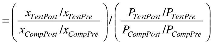
The ROR is the post- versus pre-intervention rate ratio in test product users divided by the post- versus pre-reformulation rate ratio in users of the comparator. As such, the ROR can be written as an odds ratio of counts divided by the cross-product of the observed person-time denominators.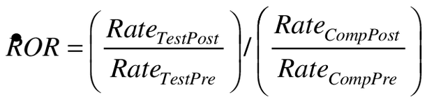
(1a)
(1b)
(1c)
The x's are counts of events, and the P's are person-time at risk in the test product and comparator groups, post- and pre-intervention. Conditioning on person-time, the large sample variance of the logarithm of the ROR is that of the logarithm of odds ratio component of (Equation 1c) [13].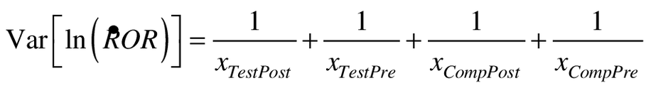
(2)
Equation 2 provides an estimate that is asymptotically the same as the one that will emerge from the maximum-likelihood estimation in Poisson regression.
At the time of planning the difference-in-difference analysis with the baseline data already in hand, the values for the x's in Equation 2 are either known (xTestPre and xCompPre ) or need to be projected to obtain power estimates (xTestPost and xCompPost ). The projected values for the post-intervention x's in the comparator are the product of: an assumed underlying temporal trend unrelated to the intervention as reflected in anticipated pre-post change in the comparator; the observed pre-reformulation rates in the comparator; and the anticipated person-time post-reformulation in the comparator:
(3)
For the test product, in addition to the underlying temporal trend in comparators, the pre-intervention rate in the test product and the post-intervention person-time in the test product, there is a further multiplier consisting of an ROR that distinguishes the trend in test product from that in comparator, assumed for the purposes of power calculation:
(4)
The distributions of the projected counts are calculated under scenarios of the assumed trend and the assumed ROR. Only the projected counts in the test and comparator groups are unknown at the time of study planning, so that for the purposes of estimating power the projected ROR under all the assumptions can be written as:

(5a)
(5b)
where:
(5c)
is an offset composed entirely of terms that have been observed at the time of planning the study.
The utility of Equation 5b is in leading to a variance of 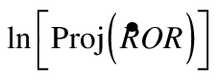 conditional on all the observed values. This differs from Equation 2 in that the large sample variance of the logarithm is that of the log-odds of future events only.
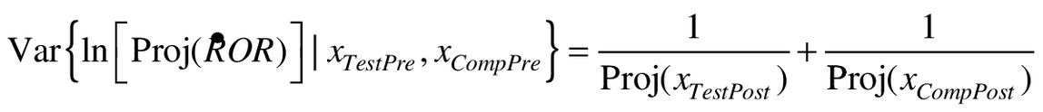
conditional on all the observed values. This differs from Equation 2 in that the large sample variance of the logarithm is that of the log-odds of future events only.(6)
Probability of excluding the null
Because the motivating example of a public-health intervention anticipates a beneficial effect, we develop the material below for an ROR <1. Anticipations notwithstanding, interventions can be harmful, and so we consider two-sided confidence intervals.
In order that the upper 1-α/2 confidence bound to ROR exclude the null, the upper bound of the logarithm of estimate of ROR must be less than 0 at the end of the study: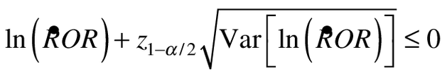
(7a)
or, equivalently: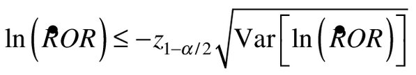
(7b)
Asymptotic normality of the log ROR estimate follows from the fact that it is a linear combination of log rate-ratio estimates, which themselves are asymptotically normally distributed with variance equal to the sum of the reciprocals of the counts of events [14]. Under normality, the probability of an estimate of ROR meeting the criterion of Equation 7b is shown in Equation 8. The power is the value of the cumulative normal distribution function up to the point  (using Equation 2 and inserting the projected values for the post-intervention x's), given a mean of ln[Proj(ROR)] and a standard deviation of
 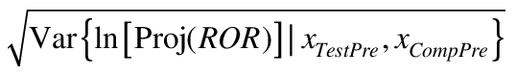 . Equivalently.
(using Equation 2 and inserting the projected values for the post-intervention x's), given a mean of ln[Proj(ROR)] and a standard deviation of . Equivalently.Power =
(8)
Equation 8 resembles the power function for any normally distributed estimator. The difference is that there are two variance estimates.  is the basis for rejection of the null at the end of the study. It incorporates the full data set, including the already-known data prior to intervention. In contrast, the term
 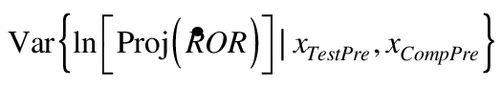 incorporates only the forward-looking uncertainty of the estimate, given what is already known.
is the basis for rejection of the null at the end of the study. It incorporates the full data set, including the already-known data prior to intervention. In contrast, the term incorporates only the forward-looking uncertainty of the estimate, given what is already known.Example
Table 1 provides information derived from two US health insurance databases [14,15]. The table records the use of OxyContin (the test product) and one of the FDA-specified comparators, extended-release (ER) morphine tablets and capsules, before and after the intervention that consisted in reformulating OxyContin, together with the number of opioid overdose events observed with each drug in the pre-intervention period as defined from the insurance-claims data [16]. Single opioid therapy was defined as the person-time when an individual received only one product.
| Pre-reformulation period (August 2008–July 2010) | OxyContin | ER morphine |
|---|---|---|
| OD events | 189 | 158 |
| Person-years of exposure | 27,827 | 19,307 |
| Crude incidence of OD, per 1000 person-years | 6.79 | 8.18 |
| Post-reformulation period (November 2010 – October 2015) | ||
| Person-years of exposure | 48,194 | 43,842 |
ER: Extended release; OD: Overdose.
Table 2 gives the conditional power for detecting a pre- to post-intervention population change in overdose rates in users of OxyContin versus ER morphine, obtained by applying Equation 8 to the data of Table 1 under different scenarios of ROR and pre- to post-intervention change in recipients of ER morphine. Figure 1 presents the same data in graphical form.
| ROR | Ratio of post-reformulation period to pre-reformulation period OD rates in the comparator (ER Morphine) | ||||
|---|---|---|---|---|---|
| 0.60 | 0.80 | 1.0 | 1.2 | 1.4 | |
| 0.80 | 24.7% | 27.9% | 30.5% | 32.7% | 34.5% |
| 0.75 | 46.3% | 53.9% | 60.1% | 65.2% | 69.5% |
| 0.70 | 69.6% | 78.8% | 85.1% | 89.5% | 92.6% |
| 0.65 | 87.1% | 93.6% | 96.8% | 98.4% | 99.2% |
| 0.60 | 96.1% | 98.8% | 99.6% | 99.9% | 100.0% |
| 0.55 | 99.2% | 99.9% | 100.0% | 100.0% | 100.0% |
| 0.50 | 99.9% | 100.0% | 100.0% | 100.0% | 100.0% |
ER: Extended release; ROR: Ratio of rate ratio.

Figure 1. Conditional power to reject ROR = 1.0 under different scenarios for true the ROR for OxyContin versus extended-release morphine and for the ratio of incidence rates between the post-reformulation period and pre-reformulation period for extended-release morphine.
ER: Extended release; ROR: Ratio of rate ratio.
Table 2 indicates that the conditional power to reject ROR = 1.0 is below 70% for a true ROR of 0.70 when the comparator overdose rates are unchanged from the pre-intervention to the post-intervention period. Apart from settings of very low conditional power, the conditional power improves in scenarios in which there is a rise in OD rates among ER morphine users from before to after OxyContin reformulation. The conditional power is lower in scenarios with a pre-post decline in OD rates among users of ER morphine. Interim calculations (not shown) for the two databases separately had shown that either of them alone would have yielded substantially lower power estimates.
The dependence of conditional power on the underlying trend in the comparator group arises from the projected counts in Equation 8, which follow in turn from Equations 5a and 5b and from Equations 3 and 4 before them. The numbers of events in both the comparator and the test product in the post period rise and fall with the magnitude of the trend in comparators. In the extreme, with a rapidly rising secular trend, the anticipated future counts will be large and relatively stable, with a small resulting variance for the projected ROR. By the same token, if the overall incidence was plummeting, the future counts would be small and the variance would be large. It would be nearly impossible to demonstrate differences between the test product and the comparator.
Figure 2 addresses the question of which among the possible comparators could be the basis for an informative analysis. The lines provide the conditional power for rejecting a hypothesis of ROR = 1 in OxyContin versus the opioid comparators for which the databases could provide information and which had arguably similar medical characteristics and usage patterns. The scenarios are for the same range of alternative ROR values as in Figure 1, all of them illustrated for a hypothesized pre-intervention to post-intervention rate ratio of 1.0 in the OD rates in comparators. ER morphine, the initially preferred comparator, has higher power at all ROR levels than any of the other potential comparators due its high volume of use. ER oxymorphone, which had a much more limited use, would be a comparator giving low power under all hypothesized scenarios.

Figure 2. Conditional power to reject ROR = 1.0 at different scenarios for true ROR for OxyContin assuming no pre-to-post change for different comparators.
ER: Extended release; IR: Immediate-release; ROR: Ratio of rate ratio.
The R program used to derive the tables and figures is given in the Supplementary Information.
Discussion
This paper has presented the changes to ordinary power calculations that are required for asymptotic conditional power calculations for a two-period design in which the changes in event rates are to be compared between a test drug and a comparator, given that the information from the ‘pre-’ period is already known, and that the denominators for the ‘post-’ period are either known or can be accurately estimated. The key is to separate out the variance of the estimate, which incorporates uncertainty in all the counts of events, from the variance of the projection of the estimate given known information, which involves uncertainty only in the elements not available at the time of study planning. In this respect, the design considerations are closely related to the analysis of conditional power.
The two-period difference-in-differences design described here is closely related to the interrupted time series design. The principal distinction is that most interrupted time-series designs in drug safety involve multiple measurements before and after the intervention, so that the slope in the secular trend in rates can be assessed, as can the step-change from the end of the pre-period to the start of the post-period. This contrasts with the ratio change in the event rates in the pre-intervention and post-intervention periods assessed in the two-period difference-in-differences design.
The two-period design for adverse event rates also resembles the pretest-posttest design widely used in social sciences [2]. A key difference is that it is not possible to condition on individual, as the occurrence of an event leads to a modification of drug exposure status or removes a person from analysis altogether. Epidemiologic designs that match on person and consider both pre- and post-event person-time depend on the assumption that the event does not affect participation or treatment status [17]. While event-dependent perturbations in exposure may sometimes be accounted for in self-controlled designs, biases arising from event-dependent censoring cannot be removed [18,19]. Even beyond event-related censoring, some individuals may contribute person-time to only the pre- or post-intervention period, and would not contribute to estimates in an individually matched analysis.
Because they involve uncertainty before and after the intervention in the compared groups, difference-in-difference designs have lower power than single-group designs, and so they may be most often carried out in very large databases such as the ones cited in the example. These, however, have become a mainstay of pharmacoepidemiologic analysis.
This presentation is not intended to replace the use of Equation 2 to create a straightforward evaluation of the point estimate and confidence bounds of the ROR estimate after a study is complete. Even when its power against a hypothesis is low, a study may sometimes generate data that are statistically incompatible with the hypothesis, so that a study with low power may produce an actionable result [20]. When the data are complete, the power analysis is relevant principally for what-if considerations of conditions other than those observed.
Future perspective
Databases of electronic records are accumulating enormous archives of secondary data relevant to public health decisions. Studies using this information will gradually abandon the traditional perspective in which all the relevant data are to be assembled after a protocol is written. Until then power calculations need to properly distinguish what is known and what is yet to be observed. In the limit, when all data are in hand and the only task is to organize them, ‘precision’ will entirely displace ‘power’ in the research vocabulary.
Power calculations need to be modified when parts of the data are already in hand.
There is a distinction between the variability in the measures on which test statistics and confidence intervals are based and the portion of the variability in measures that depends on future events.
Pre-post assessments of reformulation opioids for abuse deterrence can use baseline data that have been established already.
Supplementary data
To view the supplementary data that accompany this paper please visit the journal website at: Supplementary Material
Acknowledgements
The authors are grateful to L Li for her comments on earlier versions of this article.
Financial & competing interests disclosure
This work was supported by Purdue Pharma, LP. P Coplan was an employee of Purdue when this work was conducted. AM Walker is an employee of World Health Information Science Consultants LLC (WHISCON) and DC Beachler is an employee of HealthCore, a subsidiary of Anthem, Inc. WHISCON and HealthCore received funding from Purdue for the development of this research. The authors have no other relevant affiliations or financial involvement with any organization or entity with a financial interest in or financial conflict with the subject matter or materials discussed in the manuscript apart from those disclosed.
No writing assistance was utilized in the production of this manuscript.
Open access
This work is licensed under the Attribution-NonCommercial-NoDerivatives 4.0 Unported License. To view a copy of this license, visit http://creativecommons.org/licenses/by-nc-nd/4.0/
Supplementary Material
File (supplementary_information.docx)
- Download
- 37.33 KB
References
1.
US Food & Drug Administration. Risk Evaluation and Mitigation Strategies (REMS) (2018). https://www.fda.gov/Drugs/DrugSafety/REMS/default.htm.
2.
Bertrand M, Duflo E, Mullainathan S. How much should we trust differences-in-differences estimates? Quart. J. Econ. 119(1), 249–275 (2004).
3.
Peacock A, Larance B, Bruno R et al. Post-marketing studies of pharmaceutical opioid abuse-deterrent formulations: a framework for research design and reporting. Addiction (2018) [Epub ahead of print].
4.
Lachin JM. A review of methods for futility stopping based on conditional power. Stat. Med. 24(18), 2747–2764 (2005).
5.
Alling DW. Early decision in the Wilcoxon two-sample test. J. Am. Stat. Assoc. 58(303), 713–720 (1963).
6.
Lan KK, Wittes J. The B-value: a tool for monitoring data. Biometrics 44(2), 579–585 (1988).
7.
Lan KKG, Simon R, Halperin M. Stochastically curtailed tests in long-term clinical trials. Commun. Stat. C1(3), 207–219 (1982).
8.
Halperin M, Ware J. Early decision in a censored Wilcoxon two-sample test for accumulating survival data. J. Am. Stat. Assoc. 69, 414–422 (1974).
9.
Kittleson JM, Emerson SS. A unifying family of group sequential test designs. Biometrics 55, 874–882 (1999).
10.
Walker AM. Conditional power as an aid in making interim decisions in observational studies. Eur. J. Epidemiol. (2018) [Epub ahead of print].
11.
Wagner AK, Soumerai SB, Zhang F et al. Segmented regression analysis of interrupted time series studies in medication use research. J. Clin. Pharm. Ther. 27(4), 299–309 (2002).
12.
Oakes JM, Feldman HA. Statistical power for nonequivalent pretest-posttest designs. The impact of change-score versus ANCOVA models. Eval. Rev. 25(1), 3–28 (2001).
13.
Agresti A. Categorical Data Analysis. 3rd Edition. John Wiley & Sons, NJ, USA; Section 3.1.7, 73–75 (2013).
14.
IBM Watson. Putting research data into your hands with the MarketScan databases (2017). https://truvenhealth.com/markets/life-sciences/products/data-tools/marketscan-databases.
15.
National Institute of Health. HealthCore data description for NIH Collaboratory distributed research network (2017). https://www.nihcollaboratory.org/Pages/Healthcore-MetaData-Table.aspx.
16.
Green CA, Perrin NA, Janoff SL et al. Assessing the accuracy of opioid overdose and poisoning codes in diagnostic information from electronic health records, claims data, and death records. Pharmacoepidemiol. Drug Saf. 26(5), 509–517 (2017).
17.
Whitaker HJ, Farrington CP, Spiessens B et al. Tutorial in biostatistics: the self-controlled case series method. Stat. Med. 25(10), 1768–1797 (2006).
18.
Farrington CP, Whitaker HJ, Hocine MN. Case series analysis for censored, perturbed or curtailed post-event exposures. Biostatistics 10(1), 3–16 (2009).
19.
Farrington P. Censoring on outcome is not valid in self-controlled case series studies. J. Clin. Epidemiol. 66(12), 1428–1429 (2013).
20.
Walker AM. Low power and striking results – a surprise but not a paradox. N. Engl. J. Med. 332(16), 1091–1092 (1995).
Information & Authors
Information
Published In
Copyright
© Alexander M Walker.
History
Received: 13 June 2018
Accepted: 17 July 2018
Published online: 22 August 2018
Keywords:
Topics
Authors
Metrics & Citations
Metrics
Article Usage
Article usage data only available from February 2023. Historical article usage data, showing the number of article downloads, is available upon request.
Citations
How to Cite
Conditional power for assessing population interventions. (2018) Journal of Comparative Effectiveness Research. DOI: 10.2217/cer-2018-0053
Export citation
Select the citation format you wish to export for this article or chapter.